Introduction to computational thinking
Use 'Print preview' to check the number of pages and printer settings.
Print functionality varies between browsers.
Printable page generated Sunday, 26 July 2026, 9:40 PM
Introduction to computational thinking
Introduction
One can major [i.e. graduate] in computer science and do anything. One can major in English or mathematics and go on to a multitude of different careers. Ditto computer science. One can major in computer science and go on to a career in medicine, law, business, politics, any type of science or engineering, and even the arts.
Sounds great that ‘One can major [i.e. graduate] in computer science and do anything’, doesn’t it? Then again, isn’t this miles away from the view of computing as a training ground for programmers and system builders? The good news is that one doesn’t necessarily need to exclude the other! The grand vision behind this quote is that learning to program, build large systems, and so on, allows you to develop something which is much more valuable than any of these on their own, namely the ability to think like a computer scientist. Over the past decade or so, Jeannette Wing has been popularising this view under the banner of computational thinking.
Much of the material in this course is organised around video clips from a presentation that Wing gave in 2009 entitled ‘Computational Thinking and Thinking About Computing’ (Wing, 2009). The presentation builds on Wing’s influential 2006 ‘Computational Thinking’ paper in which she set out to ‘spread the joy, awe, and power of computer science, aiming to make computational thinking commonplace’ (Wing, 2006, p. 35).
In this course you will learn more about what computational thinking is and why it is such a desirable skill – arguably the skill for the twenty-first century.
This OpenLearn course is an adapted extract from the Open University course M269 Algorithms, data structures and computability.
Learning outcomes
After studying this course, you should be able to:
describe the skills that are involved in computational thinking
define and use the concepts of abstraction as modelling and abstraction as encapsulation
understand the distinctive nature of computational thinking, when compared with engineering and mathematical thinking
be aware of a range of applications of computational thinking in different disciplines.
1 Computational thinking and automation
To state more precisely what computational thinking is, we need to consider the ideas of an algorithm and a computational problem. We will think about these ideas in the next activity.
Activity 1 Algorithms and computational problems
Look at Figure 2. This shows page 18 of John Gough’s Practical Arithmetick in Four books, which is a tutorial maths book first published in 1767. The text under the heading ‘General Rule’ gives a description of a process for adding together three non-negative integers, each written as a finite sequence of digits. (The fact that three numbers are added is rather arbitrary: the process would work just as well for adding together two numbers or indeed any number of numbers.)
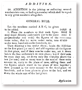
Explain whether this textual description is an algorithm according to the following description of an algorithm.
An algorithm is a solution to a problem which has three properties:
- an algorithm consists of a step-by-step list of instructions
- an algorithm is a finite process (this means it is guaranteed to finish at some point)
- the algorithm should solve any instance of the problem that might arise.
Discussion
First, we need to consider whether the text describes a step-by-step list of instructions. This is not always obvious. At some points it does and at some points it doesn’t.
At many points the text does provide instructions to be carried out sequentially, such as:
- ‘place the numbers so that each figure may stand directly underneath (…) the figures of the same value’
- ‘begin the addition at the first place’.
Although other parts of the instructions are not explicitly presented as a list of instructions, it is easy to see how the textual passage could be mapped onto such a list. In that list, certain instructions would be repeated for each of the columns involved (‘then proceed in the same manner … from place to place to the last’).
So, let’s assume that the text does have the first property. Does it also have the other two properties?
According to the second property, the process should be finite. This is indeed the case. The numbers being added will each have a finite number of digits, so only a finite number of columns will be involved, and the process only requires a small number of steps at each column.
Finally, the process does apply to any instance of the problem, where the ‘instances of the problem’ are all combinations of three integers, each represented by a finite sequence of digits in the range 0–9. The text leaves it implicit what instances the algorithm is intended to apply to.
The precise specification of the ‘instance of the problem’ can be thought of as part of the task of formulating a problem as a computational problem. By a computational problem, we mean "a problem that is stated sufficiently precisely such that one can attempt to write an algorithm to solve it."
Having met the ideas of algorithms and computational problems, let us state what computational thinking is not: computational thinking is not about us humans following an algorithm when carrying out the task of adding numbers on paper or in our head. It is not about thinking like a computer - rather, computational thinking is first and foremost thinking about computation. In particular, computational thinking consists of the skills to:
- formulate a problem as a computational problem
- construct a good computational solution (i.e. an algorithm) for the problem, or explain why there is no such solution.
A computational thinker can take a problem and state it sufficiently precisely for it to be potentially solvable by an algorithm. Once the problem has been stated in the right way, a computational thinker tries to construct an algorithm that solves it. A computational thinker won’t, however, be satisfied with just any solution: the solution has to be a ‘good’ one. We will discuss two specific properties of a good solution later on in this course: efficiency and correctness. Finally, computational thinking goes beyond finding solutions: if no good solution exists, one should be able to explain why this is so. This topic, however, takes us beyond the scope of this course into computability and computational complexity theory.
Most of the activities in this course involve watching extracts from Wing’s presentation ‘Computational Thinking and Thinking About Computing’. Remember to read through the activity before watching the video.
1.1 Automation
Activity 2 Automation, abstraction and modelling
After you’ve watched the following extract of Wing’s talk, complete this activity.
Transcript: Automation, abstraction and modelling
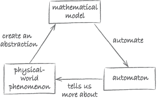
Computing! Let's first talk about computing. Computing is what I like to call the automation of abstraction. This is quite abstract and I will try and explain what I mean by this but I like to think about computing with these two ‘A’s: automation and abstraction. It really is this feedback loop that one has when you are abstracting from some physical-world phenomenon creating a mathematical model of the physical-world phenomenon and then analysing the abstraction doing some manipulations of the abstraction and in fact automating the abstraction, which then tells us more about the physical-world phenomenon that we are actually modelling. When I talk about automation and this is the whole of the talk that I am going to give so I am just going to give this as a side note. When I talk about automation I am very careful to include that the automaton can be a human or it can be a machine. After all humans compute, we may not be as fast as machines but in fact there is some ways humans are much, much better computers, than machines. In other words there are still some tasks that humans can solve better than machines. Vision is one example. Speech, natural language processing. A lot of challenges of artificial intelligence are put forth for us as scientists because machines still can’t do them as well as humans but that is just a base case. I would also like to talk about humans and machines, together, in fact, networks of humans and machines together as an automaton. So think now that you can bring together the intelligence of a human with the intelligence of a machine, networks of them, that itself is collective intelligence, that could be an automaton in my world of automation. This is quite a powerful notion, very unusual. Save that thought because I am going to come back to it at the end of my talk. As I said that is just part of the picture with respect to computing and computer science but that is really not what I am going to talk about for the most of my talk. I am really going to focus on the abstraction part of computing.
The aim of this activity is to get you to think about what Wing is saying in the following, rather long but important, sentence: ‘… this feedback loop that one has when you’re abstracting from some physical-world phenomenon, creating a mathematical model of this physical-world phenomenon, and then analysing the abstraction, doing sorts of manipulations of those abstractions, and in fact automating the abstraction, that then tells us more about the physical-world phenomenon that we’re actually modelling.’
Place the following labels in the correct positions of the diagram below. (Note: the diagram will not work with Internet Explorer 8, if this is your usual browser you will need to use an alternate browser to view the diagram.)
Discussion
It is important to have a good grasp of this diagram. It provides a high-level overview of the key ingredients of computational thinking and how they are related to each other. In the remainder of this course, we will flesh out some of the details that lie behind this diagram.
2 Computational thinking and abstraction
In the next activity you will see Wing explain how computational thinking involves the process of abstraction.
Activity 3 Abstraction
Watch the video and then complete this activity.
Transcript: Abstraction
Computational thinking is all about the process of abstraction. Let me explain what I mean by that. First of all, it is choosing the right abstraction. Not every abstraction is going to be appropriate for the problem you are trying to solve. So first you choose an abstraction and then by definition of abstraction are ignoring irrelevant detail and encapsulating in this abstract model the details of importance. That means I’m immediately talking about at least two levels of interest. The level I am ignoring the detail from and the level of interest so the abstraction process immediately means that you are talking about at least two levels of abstraction, and in fact the way in which computer scientists deal with scale and complexity in the kind of artefacts that we build and design is through layers of abstraction. That allows us to focus at each layer only on the properties or behaviours of interest and then we build these complex systems by layering or other means of composition. So when we talk about abstraction it’s not just the abstraction or the particular model. It’s the layers and also the relationships between the layers and because we usually define these abstract models in very precise terms, mathematical terms, we are able to define the relationships between these layers also precisely in mathematics. In fact all of what I said is as we do in mathematics. After all it is not that computer scientists invented abstraction. Mathematicians and scientists use abstractions all the time. What’s different is that in computing we are always operating at least two layers of abstraction at the same time and we are very formal about the relationship between the two layers.
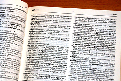
Wing talks about abstractions as a means of ignoring detail that is not of interest. Consider the following description of an algorithm for searching a paper and ink dictionary.
Given:
- i.a dictionary
- ii.a headword W which appears in the dictionary
to find the definition of W:
- Begin the search with an entry that appears (roughly) in the middle of the dictionary. Then there are three possibilities:
- The current entry’s headword is W. In this case, the definition of W is the definition of the current entry.
- W appears alphabetically before the current entry’s headword. In this case, the entry with headword W must appear in the first half of the dictionary. Look for the word W, following the same approach, in the first half of the dictionary.
- W appears alphabetically after the current entry’s headword. In this case, the entry with headword W must appear in the second half of the dictionary. Look for the word W, following the same approach, in the second half of the dictionary.
This is an informal description of an algorithm, but the steps are sufficiently precise that a human should have no problem following them. This algorithm depends crucially on the fact that the words in a dictionary are alphabetically ordered. It also, however, ignores some of the details of paper and ink dictionaries. Can you list of few of these?
Discussion
Details of a paper and ink dictionary that come to mind include: the size and thickness of its pages, the colour of its cover and the size of the printed font. None of these played a role in the algorithm that is described above. Perhaps the most salient abstraction relates to the fact that paper and ink dictionaries are made of pages. They are not simply a list of words and definitions. Rather, the words are distributed across the pages of the dictionary. The algorithm doesn’t take into account the distribution of the words in a dictionary across pages: for example it would work equally well with a dictionary printed on a single, enormously long paper scroll.
Wing’s discussion of abstraction draws on a wide variety of concepts. You have come across phrases such as ‘ignoring’ and ‘hiding information’, ‘levels’ and ‘layers’, ‘models’ and ‘implementation’. It has been left somewhat in the air how these all hang together. So next, we will make the relations between them explicit. To do so, we will distinguish between two kinds of abstraction:
- abstraction as modelling
- abstraction as encapsulation.
Although Wing deals in great detail with the idea of abstraction as modelling, she only hints at the concept of abstraction as encapsulation. Both are, however, at play in computing. Distinguishing between them will give you a better understanding of the remainder of Wing’s story.
2.1 Models
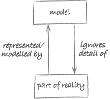
Let us think more generally about the abstraction depicted in Figure 5. For this purpose, we will be using the diagram in Figure 6. Instead of Wing’s somewhat unwieldy expressions ‘mathematical model’ and ‘physical-world phenomenon’, we will use the shorthands ‘model’ and ‘part of reality’.
The diagram in Figure 6 shows that abstraction as modelling can be understood in terms of the relationship between a part of reality and a model which represents the details of interest of this reality. For this reason, models are sometimes also referred to as representations.
For the purpose of the current example, the part of reality that we’re interested in is the paper and ink dictionary of Activity 3. The algorithms in Section 1 for looking up words work with a model of a dictionary as an alphabetically sorted list of headwords, each paired with its definition. The model corresponds to how the data that the algorithm works with are structured. This model captures the essentials (i.e. that the dictionary consists of an alphabetically sorted list of words and their definitions) and ignores certain details (for example, that a physical dictionary is divided into pages of a certain size and has a cover to protect it). In other words, the irrelevant details are not reflected by the structure of the data that the algorithm works with.
Activity 4 Representations
Representations, including paintings and drawings, are models. This is brilliantly illustrated by René Magritte’s famous painting of a pipe with the words ‘Ceci n’est pas une pipe’ (‘This is not a pipe’) underneath (Figure 7). Explain how this painting brings home the point that modelling involves two levels: the abstraction and the reality which the abstraction models.

Discussion
When looking at this painting, my initial thought was: ‘Look, a pipe – why does it say in French that this is not a pipe?’ Then it dawned on me that of course this is indeed not a pipe: it’s merely a painting of a pipe. With this painting, Magritte reminded me that representations usually involve two levels: in this case the painting of a pipe and a real pipe on which the painting is based. The former is an abstraction which ignores some of the properties of actual pipes (for example, that they have a smell, usually of tobacco). Interestingly, the title of this painting is La trahison des images (The Treachery of Images).
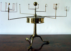
The part of reality for which one creates a model or representation doesn’t need to be a static object such as a pipe or dictionary. It can also be a process or system which changes over time. In that case, the model will not only have to capture any enduring properties of interest, but also any changes in time that are of interest. For example, in astronomy there is a rich tradition of building such models of the solar system (see Figure 8). The purpose of such a model, known as an orrery, is to represent the position of the planets relative to each other over time.
The invention of the orrery is usually attributed to George Graham (1673–1751). Graham worked on this with the support of the 4th Earl of Orrery, which explains the name. The tiny crank on the side of the central cylinder in Figure 8 allows the model to be animated. Turning the crank causes the (representations of the) planets to follow a path around the (representation of the) Sun at the centre of the model. Usually such an animated model is referred to as a simulation.
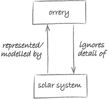
As with any model, an orrery ignores certain details of the part of reality that it models. For example, compared with the scale of the distances between the planets, the planets are too large. The relationship between the solar system and an orrery is as depicted in Figure 9.
2.2 Encapsulation
The model of the solar system in Figure 10 also illustrates the second type of abstraction: abstraction as encapsulation. The brass cylinder in the middle of the device encloses a clockwork of cogwheels similar to the one in Figure 10.
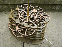
This mechanism causes the small spheres representing the planets to rotate around the centre at a velocity that is proportional to the speed of the actual planets. The mechanism is hidden from view for the casual user, who is only interested in the movement of the planets. Figure 11 illustrates this other view of the orrery in terms of two layers.
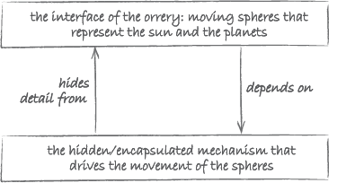
Generally, abstraction as encapsulation involves the two layers shown in Figure 12.
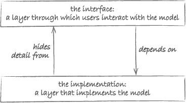
The layer through which the user interacts with the model is called the interface. It hides the detailed workings of the model from the user. The interface sits between the user and the layer at which the model is implemented. The latter is responsible for making the model do what it is supposed to do. This is where the automation of the model takes place.
2.3 Encapsulation in computing
Abstraction as encapsulation is common everywhere in computing. Sometimes it is referred to as ‘abstraction as information hiding’ (instead of encapsulation).
Let us consider an example. Our example will make use of the Python programming language. This language is used throughout M269 Algorithms, data structures and computability on which this OpenLearn course is based. It was chosen because it is eminently suitable for learning the basic concepts of computer science and programming. It allows you to write concise, easily understood programs. You should be able to follow most of the following discussion if you have had some experience with an imperative programming language.
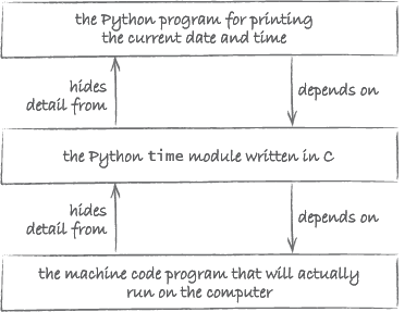
The incredibly short Python program below will display the date and current time (see Figure 13). It depends on a built-in Python module which is imported in the first line.
import time
print(time.ctime())
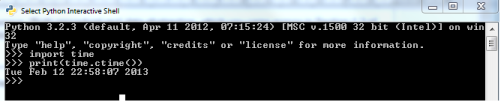
How does time.ctime() work? We don’t know and we don’t need to know! Someone has written the time module and documented its interface, which contains the function ctime(). We can just use the function without any knowledge whatsoever of its implementation.
However, under the bonnet the time module is itself a program, written in C, another high-level programming language! The programmers of the module, when they wrote it, only needed to know C. They were able to ignore the details of the low-level machine language that the C program would get translated into.
So now we have three layers of programming abstraction (Figure 14).
Think about it: if layers of encapsulation did not exist, the short and easily understood program to display the time (above) would be impossible. We would have to deal directly with instructions written in machine language. There would be many of them and they would be in a language which is very hard for humans to understand.
Programming abstraction doesn’t stop there. We can define new abstractions of our own. For example the following function prints the n times table up to 9 times n.”
def timesTable(n):
for m in range(1, 10):
print(m, 'times', n, 'is', m*n)
Once this function is defined we can call it whenever we like without having to bother again with the details.
timesTable(9)
In fact we can create a Python module that encapsulates this function, so the detail is completely hidden! Suppose we name the module demo. Then the timesTable function can be used from a different Python program, like this:
from demo import timesTable
timesTable(7)
But now we can define a new function that depends on timesTable. The function printUsersTimesTable below prompts the user for a number and then uses timesTable to print the corresponding times table (see Figure 15).
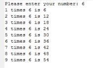
def printUsersTimesTable():
aNumber = input('Please enter your number: ')
timesTable(int(aNumber))
So we can build a hierarchy with any number of layers of abstraction, with the detail of each layer hidden from those above and each layer – apart from the bottom one – interacting with the layer below via its interface.
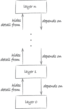
The overall picture that emerges is one of a hierarchy of layers. As illustrated in Figure 14, in such a hierarchy Layer 0 hides its details from Layer 1 above it, Layer 1 hides its details from Layer 2, etc. Conversely, Layer 1 depends on Layer 0, Layer 2 depends on Layer 1, etc.
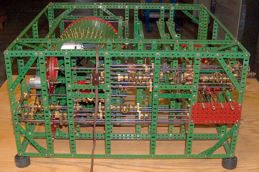
Figure 14 also shows that such a hierarchy eventually bottoms out at Layer 0. That is the layer at which the abstraction is implemented in physical reality, i.e. a substrate/hardware. This physical layer constrains what is possible at the layers that are built on top of it. Nowadays, most computers are built using electronic components. This is, however, by no means the only possible physical substrate. When Charles Babbage (1791–1871) designed the first programmable computer, he came up with a steam-powered machine built of brass and iron. Babbage never finished his machine, but recently part of it has been constructed using Meccano (see Figure 17).
Without going into detail, the idea of layers of abstraction in computing is not restricted to programming languages. It extends, for example, to operating systems and computer networks. In both, a distinction is made between physical and logical layers. Actual devices (e.g. hard drives and computers) and networking hardware (e.g. copper wires) are part of the physical layer. The logical layer contains abstractions (such as IP addresses and protocols).
2.4 Why modelling and encapsulation matter
Both abstraction as modelling and abstraction as encapsulation allow us to manage complexity:
- In the case of modelling, this is done by discarding information: we abstract away all that is irrelevant, to leave a model that contains only what is actually of interest.
- In the case of encapsulation it is done by hiding information: we encapsulate the details of an implementation/automation (of a model) behind an interface.
These strategies are utterly essential to all computer modelling. Without modelling we would be swamped by the complexity of the real world and it would be impossible to define the problem precisely enough to allow it to be solved using an algorithm. Without encapsulation we would be swamped by the detail of the ‘computer world’ and would find it impossible to deal with the complexity required to implement algorithms as computer programs.
Activity 5 Modelling and encapsulation
In answer to Activity 2 you were asked to construct the diagram in Figure 18. Describe where modelling and encapsulation fit into this diagram.

Discussion
Modelling is involved when one creates an abstraction for a physical-world phenomenon. Modelling results in a mathematical model which can then be automated. To deal with the complexity of automating a model, one can use encapsulation.
2.5 Computational thinking: the overview diagram
The aim of this subsection is to draw together some of the concepts you have encountered so far. Consider once more the diagram illustrating some of Wing’s ideas (Figure 19).

The three main components in the diagram are:
- a physical-world phenomenon
- a mathematical model
- an automaton.
How do these relate to the concepts you met in Section 1, namely:
- real-world problem
- computational problem
- algorithm and data structures?
Let us start with Wing’s use of the term ‘mathematical model’. As we will now explain, Wing’s notion of a mathematical model is linked to that of a computational problem. According to Wing, a mathematical model is an abstraction of the physical-world phenomenon of interest. It ignores irrelevant detail. It also is the point of departure for automation. The fact that it is a mathematical model means that it is sufficiently precise to be used as a starting point for creating an automaton. Now, you may recall that we defined a computational problem as a problem that is expressed sufficiently precisely that it is possible to attempt to build an algorithm to solve it. In other words, Wing’s mathematical model is nothing other than a computational problem.
Wing’s physical-world phenomenon is abstracted by the mathematical model, just like a computational problem provides an abstraction of a real-world problem.
Algorithms and data structures form the link between a computational problem and its automation. Finding algorithms and data structures is part of automating. When these are then implemented as a program and executed, they provide a machine that solves the problem. In Wing’s words, the resulting machine – or automaton – automates the abstraction.
The complexity of the machine, as we have just discussed, is managed by having a series of encapsulated layers.
To sum all this up, we can refine the diagram of Figure 19 as shown in Figure 20.
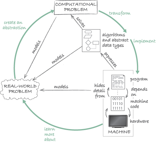
Whereas the core of this diagram represents artefacts (real-world and computational problems, machines) and their relations (models, solves, and expresses), the green arrows indicate the actions that a computational thinker engages in (i.e. create, transform, implement and learn).
2.6 Varieties of abstraction
In the next video clip, Wing compares and contrasts abstraction in computational thinking with abstraction in mathematics and engineering. In the following activity you will make these comparisons explicit.
Activity 6 Computational, mathematical and engineering thinking
Parts 1-8
Watch the video and complete the activity by ticking the appropriate boxes.
Transcript: Computational, mathematical and engineering thinking
So this isn’t anything new from what mathematicians do but in computing we don’t just invent abstractions for the beauty and elegance of the abstraction as mathematicians tend to strive for. We have other concerns that constrain the abstractions we choose. So in particular I would like to talk about the measures of a good abstraction in computational thinking. The first and foremost typical question a computer scientist would ask is, ‘how efficient is this. Is this the most efficient way to solve the problem’, and when I talk about efficiency I talk about it in terms of space and time. Is this the fastest way to get from here to there? Is this a procedure which is going to require the least amount of space for that space and time? And I think what is most interesting right now is there is a lot of interest in what I would call the third dimension of analysing the complexity of the kinds of abstractions that we invent and that has to do with energy. There is so much interest now in a society and the administration on energy and I think of computing as a discipline needs to revisit a lot of the abstractions we have invented already in terms of this third dimension. So for those of you who are researchers in computer science I advocate that we are going to have to throw out all our algorithm text books and rewrite them all in terms of these three dimensions now. The other measure of goodness for the abstractions that computer scientists like to invent is correctness. After all when you are writing a program or building a system you want it to do the right thing and so we always ask not only how fast does this, say algorithm, perform but does it do the right thing? And what does, does it do the right thing mean? We usually ask does the program compute the right answer and asking that question alone opens up a lot of research questions. But we also wanted it to do something useful so it is not enough that it does the right thing we actually want the answer to be spit out eventually and that is the question, does the program produce an answer? There are complexity results that show that this is not always an easy question to answer, and then of course there is the other ‘ilities’ if you will when we look at a particular abstraction and judge whether it is good or not. Simplicity and elegance as we have for mathematics, usability, modifiability, maintainability, cost and so on. Now if you look at this list you will say, well that is no different from good engineering, and so in fact computational thinking or computing very much draws on mathematical thinking and draws from engineering thinking and comes together in terms of the automation of the kinds of abstractions we build. What I would like to … I promise that I will say a few more high level remarks and then I will get into some concrete examples. But I like to think that computational thinking really does draw on mathematical and engineering thinking, it draws on mathematics certainly as its foundation but we in computing are unconstrained by the physics of the underlying … we are constrained by the physics of the underlying machines. So, in the end there is going to be some machine or there is going to be some human brain and we are in terms of what we can execute or automate are going to be constrained. So a typical computer like this is going to have finite memory, it can only go so fast and so it is constrained by the physics of this device. The brain scientists are trying to understand the physical and intellectual limitations of our brain as an automaton. Computational thinking certainly draws on engineering since our systems interact with the real world. However we in computing can build virtual worlds, worlds that are unconstrained by physical reality and so when you interact in a virtual world. So how many people have heard of second life. Second Life is a virtual world which you can enter and this virtual world defies the laws of physics. You have avatars who fly around, you have corpse-like beings that die and come alive again. That’s not like in the real world so what is it in computing that enables this kind of defying the laws of nature, building worlds that are virtual. It’s the software. Software enables these physical devices to be beyond the real world. When I talk about computational thinking, I really mean the concept and not the artefact that computer scientists produce. This is a little abstract, I promise to get a little more concrete. And finally, I talk about computational thinking as being something for everyone everywhere. It will be a reality when it is so integral to our endeavours that it disappears as an explicit philosophy. So being more specific, here is unfortunately a laundry list of what I would say computational thinking concepts and those of you who are computer scientists or engineers or mathematicians will recognise many of these classes of abstractions. What I mean by putting this list down is not for all you to understand all this of this, but just to say that I distinguish between computational thinking and computer literacy, that is how to use Word, or Excel, PowerPoint. Computational thinking is not that and I distinguish between computational thinking and computer programming because computing is a lot more than computer programming. Ideally I could come up with a better list if you will rather than this potpourri of concepts. I’m actually working on that as I speak.
a.
Computational thinking
b.
Mathematical thinking
c.
Engineering thinking
The correct answers are a, b and c.
Discussion
In all three disciplines, the use of formal/mathematical notation is common:
a.
Computational thinking
b.
Mathematical thinking
c.
Engineering thinking
The correct answers are a and c.
Discussion
Mathematics typically works only with a single layer: there is no distinction between the ‘properties of interest’ and the ‘ignored detail’. The abstraction is studied in its own right, without reference to some other layer which it represents. Of course, this is an idealisation. Many areas of mathematics did start as a representation of some aspect of the real world. For example, geometry began with Euclidean geometry, which was intended as a model of physical space.
Both engineering and computing rely on at least two layers. At the basis, there is a layer grounded in the real world. This is the layer in which the problem of interest lies (for example a bridge or car in engineering). In addition to this layer, there is at least one further layer which ignores certain of its details. For instance, an engineer may use mechanics to calculate the forces operating on a bridge when a car crosses it. In doing so, the engineer will abstract away (or ignore), the colour in which the bridge is painted, the brand of the car, and many other things that are not relevant for calculating the forces in question. We’ve seen that a computer scientist who simulates a dictionary may, similarly, ignore certain properties of a physical dictionary.
a.
Computational thinking
b.
Mathematical thinking
c.
Engineering thinking
The correct answers are a, b and c.
Discussion
In all three disciplines, beauty and elegance are criteria that are used to compare competing abstractions. These are, however, more central in mathematics, where the abstraction is often judged in its own right, without reference to an underlying reality that it represents.
a.
Computational thinking
b.
Mathematical thinking
c.
Engineering thinking
The correct answers are a, b and c.
Discussion
In connection with this criterion, Wing asks in particular: ‘Does it do the right thing?’ and ‘Does it do anything?’ These questions are clearly relevant for both computational and engineering abstractions. It is perhaps less clear what they mean in the context of mathematics. Arguably, since mathematics is about the abstraction itself, one can’t really distinguish correct from incorrect abstractions because there is nothing to compare them with. However, even when dealing with pure abstractions, we may want to make sure that they are consistent. A mathematical theory that states that a mathematical object both does and does not have some property would be in violation of this criterion (e.g. a theory which says that two lines cross and do not cross each other).
a.
Computational thinking
b.
Mathematical thinking
c.
Engineering thinking
The correct answers are a and c.
Discussion
In connection with computing, Wing mentions three dimensions of efficiency: time (how fast?), space (how much space?) and energy (how much power?). Each of the three efficiency criteria can also be applied in engineering contexts (e.g. how fast can the engine run, how much space does it occupy, and how much energy does it consume?). None of these considerations has a clear equivalent in mathematics.
a.
Computational thinking
b.
Mathematical thinking
c.
Engineering thinking
The correct answers are a and c.
Discussion
All of these practical considerations are important in both engineering and computing contexts. They are not directly applicable to mathematics.
a.
Computational thinking
b.
Mathematical thinking
c.
Engineering thinking
The correct answers are a and c.
Discussion
Both engineering and computing are constrained by physical reality. For example, the classical model of computing uses the bit (0 or 1) as the basic unit of information. It is constrained by whichever physical means is used to represent a bit (whether it be an electrical current or, for instance, the position of a mechanical lever). The physical hardware constrains, among other things, how quickly the state of a bit can be changed (from 0 to 1 or vice versa).
a.
Computational thinking
b.
Mathematical thinking
c.
Engineering thinking
The correct answers are a and b.
Discussion
Mathematics, as the study of pure abstractions, is independent of physical reality. Computing, though always constrained by the physical layer at which the hardware operates, allows us to build on top of the hardware layer software layers that model non-existent realities. By automating these virtual realities, it allows us to see and even experience realities that go beyond what is physically possible.
2.7 Virtual worlds
Though engineering and computing have much in common, Wing argues that one big difference between the two is that computing allows us to escape from the constraints of the physical world. First, however, she points out that automatons (i.e. entities that carry out automation) are constrained by physics in the sense that they require a physical substrate/hardware to exist and work. In the end, any algorithm can only run on a real machine – a machine made of hardware – whether it comprises electronic components, brass and iron, or brain tissue.
Let us pursue the idea of how computing allows us to step outside the realm of physical constraints. For that we need to revisit the idea of abstraction as modelling. You have seen that algorithms can work with abstractions of real things such as paper and ink dictionaries. Perhaps more spectacularly, algorithms can also work with abstractions of things that do not exist, at least not in the physical world around us.
Activity 7 Abstractions of the non-physical
Can you give an example of an algorithm that works with abstractions of non-physical things? Hint: You can find such an example in Section 1 of this course.
Discussion
You saw an example in Section 1 when you learned about the algorithm for column addition. This algorithm works with non-negative integers. At first sight, it might seem that integers are physical objects. After all, can’t we write them down using pen and paper? Recall, however, Activity 4 (Ceci n’est pas une pipe). In that activity you studied the distinction between representations/abstractions and the reality they model. When you write down a ‘2’ (or any other number) on a piece of paper, this is a representation of the number 2, not the actual number. Why? Suppose that what you wrote down was the number 2 itself. In that case, if you erased it, 2 would cease to exist, and if you copied it, you would have created another number 2. That would be absurd! When you write down a ‘2’, this is merely a representation, not the actual number. Other people can write down a ‘2’ as well, and thereby talk about the same number that you’re talking about when using a ‘2’.
Perhaps this has set you wondering what numbers are, if they aren’t physical objects. Unfortunately, philosophers have been at loggerheads about this question since the ancient Greeks started discussing it. Many mathematicians subscribe to a view championed by the philosopher Plato (429–347 BCE), who proposed that numbers exist, but not in space and time; rather they inhabit what is known as ‘platonic heaven’.
Wing gives a further example of abstractions in computing that model something (physically) non-existent. She discusses virtual worlds, such as Second Life, a three-dimensional virtual world populated by avatars. Avatars are computer-animated characters that are controlled by real people – computer users. The avatars can do many things that we are familiar with in the real world, including walking around, talking to people, and interacting with objects. They can, however, also do things that are not possible in the real world, such as teleport from one location to a geographically distant other location. This is another instance where the automation of abstractions allows us to go beyond the things that can exist in the physical world. Note the big difference here between computing and conventional engineering. Engineers are generally interested in creating artefacts that are physically possible – what would be the point of designing a bridge that cannot be built?
3 Computational thinking everywhere
At the very beginning of this course, computational thinking was presented as a desirable skill – arguably the skill for the twenty-first century. Why? Well, in recent years, computational thinking has led to exciting developments and discoveries in a number of fields. This has caused a demand for people with computational thinking skills to move these fields forward even further. In this section, you will encounter some of these applications of computational thinking. Watch the videos, but don’t worry if you can’t follow all of it. We want you to get a feel for the big picture – you’re not expected to remember everything in detail.
Activity 8 Computational biology
Watch the following video.
Transcript: Computational biology
So now what I wanted to do is convince you that computational thinking has already influenced other disciplines. So let’s start with one discipline influenced by many different computational methods or concepts. So who can guess what that discipline might be? Don’t be shy. Scream out the answer, scream out any answer. Yes sir – that is an interesting answer. I’ll come back to that one. Medicine – is close to my answer. Biology, biology – that is my answer. It is just an answer. Computational thinking has greatly influenced biology to the point now that we have biology and computer sciences working together hand-in-hand but more than that we have now started to produce a new generation of computational biologists. Hold on, you are now answering my next question. My next question is; what was the tipping point, at which point did the biologist look over their shoulder and say, ‘you computer scientists have something to bring to the table. You computer scientists are making me think differently, making me approach my problem in a new way.’ Answer is … right, it was the shotgun algorithm that expedited the sequencing of the human genome that all of a sudden caused a lot of interest by the biologists, by the whole medical and biological communities who said hey there is something to computer science, to algorithms, more than just processing power. That is the point I am trying to make. That computing is more than just about devices and horsepower, and supercomputers, and this particular algorithm was what I think the tipping point when biology and computer science came together. Since then, there have been many, many examples of different kinds of computational methods, different kinds of computational models, different kinds of computational languages, different kinds of computational approaches for understanding biology. I have just listed a few. A lot of this is just buzzwords, if you will.
Activity 9 Model checking
Watch the following video.
Transcript: Model checking
I want to be slightly a little more technical in this part of my talk that’s not the shotgun algorithm, so I am going to go through one example that is not the shotgun algorithm to show a different kind of computational model and thinking that has influenced biology, and this is very recent work. So to do that you have to bear with me for a few slides because I am going to go into a slightly more technical part of my talk and I going to do a primer on this particular computational method, and its called model checking. I always in my talk at this point ask the audience … how many people have heard of model checking? I am surprised. After this slide you will all know what model checking is, at least in the abstract. OK, so let me go through it. There is a black box, it’s called the ‘model checker’ and it has two inputs. One is a finite state machine – what that means is that there are states and those are circles and there are transitions between the states, those are the state transitions, the lines, the arrows. And, what makes this a finite state machine is that there are a finite number of circles, finite number of states. OK, so that is one input and that is critical for this technique that it be finite. The second input is a property that we would normally write in English but, because computers can’t understand English well enough yet we write it in a more formal language. I picked this particular logic, its called Temporal Logic, it doesn’t matter, it is a formal language, a mathematical language that can reason about the ordering of events. So basically you have these two inputs, and what happens is, you describe the system of interest using this input and you describe a desirable property using this input. So you might want to say something like … when you go to the ATM machine, eventually I get my money out. So you would say … describe the ATM machine in terms of the finite state machine and all the kinds of things you could with it. Like; put your card in, punch buttons, deposit money, withdraw money and you would describe the property of ‘eventually getting my money out’ in terms of here and ideally for any ATM machine you would like to know that this property holds. OK ideally. That’s how we like to design our systems. Of course we know in reality there are always bugs. OK so those are the two inputs. The output is ‘yes’, every single ATM is designed, will always give your money back but, more realistically you will say ‘no’, here is a bug in this ATM machine, not only is there a bug but here is an example of a sequence of steps that you will take in terms of that machine where you are not going to get your money back. OK and that is called the Counter Example. So that is my primer on model checking. Basically it has two inputs, you press the button and out will say, yes, every single time you interact with the ATM machine this property will hold or, no, you will get into trouble if you do this sequence of events. OK? That is a particular computation model, computational concept, computational approach and it has been used in fact very successfully for hardware design, companies like Intel, HP, Fujitsu, IBM, they all use this kind of technique for verifying and debugging hardware/processor design. This is almost a ‘bread and butter’ kind of technique in computing. Let me … I’m going to skip that … for those of you who are interested in the formal definitions that is what it looks like. OK there are many efficient algorithms and many efficient data structures that allow us to push a button and get that black box answer. What does that have to do with biology? Well for the face of it absolutely nothing! It certainly wasn’t invented because there was a biological problem to solve. But it turns out that when you put computer scientists and biologists together or when you have a person trained in both biology and computer sciences sparks will fly and that is exactly what happened to that particular person who worked in this intersection of computer science and biology, particular model checking and protein folding and he represents a protein that has three residues in this particular case in terms of this very simplistic finite state machine where you could imagine where this state with three zeros (000) represents the folded state and this state with the three ones (111) represents the unfolded state and these numbers in parenthesis represent how much energy does it take to go from this state to this state, where you are unfolding one of the residues. OK, and so the question is what are all the paths, the ways in which this protein can unfold itself and what are the paths in which the protein can unfold itself using the least amount of energy. So now this is a very simple example, you can probably figure this out in your head, right, but suppose you had 76 residues? You couldn’t even write that out on a piece of paper! There is actually where the scale of computers come in handy because they can do that sort of calculation, no problem. So in fact they show that you can use this modelling checking technique to explore state spaces as large as 2 to the 76th using this kind of particular model-checking algorithm/model-checking approach, and this technique, it’s a pretty recent result, you see its 2007, with 14 orders of magnitude greater than comparable techniques. So this is already new stuff that we are talking about protein folding and so on but here is where you can see sparks fly when you bring computational methods to these kinds of biological problems. OK, so I promise this is the most technical part of my presentation. So that’s one discipline, many methods …
3.1 Machine learning
Machine learning is a technique for automatically finding patterns in large amounts of data. Watch the following video extract in which Wing discusses several applications of machine learning.
Activity 10 Machine learning
Transcript: Machine learning
So let’s flip it. How about one method that has influenced many disciplines? So I actually have to call on any computer scientists in the audience to help me answer this one, because I doubt the general public would know the answer. But I know there are some computer scientists in the audience so I challenge you. What method do you think has influenced so many disciplines today? – conceptional modelling – Of course I have the answer I want you to say. The answer is ‘machine learning’. How many people have heard of ‘machine learning’? More people have heard about ‘machine learning’ than ‘model checking’ so that’s good. So machine learning has completely transformed the whole field of statistics. In fact there is a whole department of machine learning at Carnegie Mellon, if you can believe that within the school of Computer Science and it’s made of faculties from Computer Science and Statistics and what they really do is Statistical Machine Learning. Another example is that there are departments of statistics now at universities for instance Purdue which has an excellent Statistics department who are hiring computer scientists because they see their future as in this combination of statistics and computing particularly in Statisitical Machine Learning. So we are seeing this in the next generation if you will. So let me give you some examples of where machine learning has influenced many, many fields. So in the sciences it is a technique that has been used to discover new brown dwarfs and fossil galaxies. This is really new scientific discoveries because of this particular technique. In medicine it has been used for discovering and inventing these kinds of drugs and uses in these applications. In meteorology: for tornado formation. In the neurosciences for understanding the brain, so I should at least give you a one sentence definition of Machine Learning given that many people may not know it. What it is, it’s a technique that allows you to analyse huge data sets, large amounts of data and find patterns and clusters in large amounts of data. So in this particular case what you feed this algorithm is lots and lots of fMRI scans, (scans of your brain). What they are able to do through using Machine Learning is to find out what part of your brain lights up when a subject sees a noun versus a verb or this kind of adjective versus that kind of adjective and it’s looking at lots and lots of fMRI scans that allow you to see those clusters, those patterns. Machine learning has been used beyond science and engineering, so for instance it is used in detecting credit card fraud. It’s used on Wall Street, (the answer from the back of the room). When you go to the supermarket and you hand the clerk your Safeway card, your affinity cards, they are tracking your purchases and the coupon you get out after your receipt, is using that kind of analysis of large amounts of data. Recommendation Systems and Reputation Systems like Netflix when you go to Travelocity to find out what customers use and so on. Machine learning is even used in sports, so I don’t know what basketball player this, is but maybe you do, but what they did was videotape lots of professional basketball players and then the coaches would use Machine Learning to find out what are the skills of these professionals so they can teach those skills to their own students. This is Lance Armstrong who used Machine Learning to analyse the kind of data he kept of himself. As you know, he is a machine – and he was quite mathematical and analytical in his training so that he could really hone his skills.
Wing gives the example of basketball coaches who use machine learning to find out which skills distinguish good players. Once they know this, they can teach those skills to their own players. Machine learning makes this possible by automatically finding patterns in the behaviour of professional players from a large collection of video recordings.
Describe this use of machine learning in terms of abstraction as modelling.
Discussion
One can view this use of machine learning as an attempt to automatically build a model of a good basketball player. Such a model is an abstraction that needs to capture the skills that distinguish a good player and ignores anything else. At a different level, machine learning is itself based on a model of learning by humans or animals. Being an abstraction, it ignores many of the details of human and animal learning, while preserving some key properties (in particular, the idea that one can learn from examples).
Activity 11 Chemistry, physics, economics …
Watch the following video.
Transcript: Chemistry, physics, economics...
In chemistry computational methods, computational concepts have been used to actually invent new molecular structures that would have desired chemical properties. In physics, (this is one of my favourite examples), I am going to labour on this a little bit in quantum computing. There is a very young professor in MIT who works in quantum computing, he’s actually in the Computer Science department but he works as a physicist. In computer science, there is a kind of quantum computer where you can represent the problem in terms of a, let’s call it a graph, but you can solve the problem if you can morph this graph into some other representation/other graph. You can solve it more easily in this second representation, and so the idea is then how can you get this graph to be morphed into this graph. There is a procedure that you can use that would allow you to make manipulations of each graph until you finally come in the middle, and have that intermediate. Physicists know about this kind of quantum computer. So, the question that quantum scientists asks, is how fast you can do this? This is something that computer scientists ask all the time, how fast can you do it, right? I already said that is the question they always ask about efficiency in terms of space and time. The physicist never asks that question of themselves, they just know that there exists some path such that you can do that, but they didn’t ask, how fast can you do it? Now again, for the computer scientists in the audience, the reason this was such a tantalising question to answer, is, if it turns out that the convergence is polynomial it means that you might have an answer to the P=NP question. So you can see why this young computer scientist at MIT would very much like to know the answer to that convergence question, and it turns out that it goes really, really, really fast until this very small window where it is exponential. Even so it was a very interesting question to pose and now he tells me that the physicists are going around asking how fast on all their convergence questions. This to me is a deep way of computational thinking influencing other people’s thinking because you ask these basic questions that we would ask, and had the answer being polynomial then wow!, what a break through in computer science. We see it in Mathematics, we see it in Engineering and I think we are going to see more of it in all other fields. In society like Economics, right now, in fact tomorrow and Friday there is a workshop at Cornell on computer science and economics that an assessor is helping to sponsor and we are seeing a lot of the theories of economics and models of economics. In fact, we already know that some of them are not applying to our real world, but they are certainly not necessarily applicable to say to the internet and internet economics, and so there is all of a sudden this new interest, completely new interest, in revisiting economic models and theories in terms of computing models and vice versa. So for instance we are very much using game theoretic models in looking at lots of problems in computer science, game theory from economics, but many of the direct relationships between economics and computer science has to do with things like added placement and keyword auctions and so on. So for instance when you type into Google and you do a search, maybe you realise to the right of your search you have all these ads, well companies actually bid on where they want their company to be listed in that list of ads. You pay a lot to be listed number 1. But maybe it doesn’t matter to be listed number 1 or 2, you pay a little less to be listed number 2, you are still number 2, you are up there, right so that the kind of game theoretic thinking that people are doing in computer science. In Law we are seeing computational thinking and in the Humanities. Again in the sense of digging into the data challenge is analysing lots and lots of data.
Conclusion
The underlying theme of this course has been ‘computational thinking’. We’ve defined this as consisting of the skills to:
- formulate a problem as a computational problem
- construct a good computational solution (an algorithm) for the problem, or explain why there is no such solution.
We introduced the idea of an algorithm with two examples: an algorithm for addition and one for dictionary search. You learned about the concept of abstraction and its two varieties: abstraction as modelling and abstraction as encapsulation. We contrasted and compared computational thinking with both mathematical and engineering thinking. You have also been shown the ‘bigger picture’: the way that computational thinking is shaping research in many disciplines, ranging from biology and physics to economics and sport science.
Glossary
- abstraction
- provides a handle on complexity by either ignoring detail by means of a model, or hiding detail through the use of encapsulation.
- algorithm
- A precisely stated, step-by-step list of instructions.
- data structure
- A way of organising data for use by an algorithm.
- encapsulation
- Hiding details of an implementation from users. This is achieved through an interface that sits between the user (or client) and the implementation.
- interface
- An interface sits between a user (or client) and an implementation. It hides the details of the implementation from the users or clients of the implementation. (See encapsulation.)
- model
- A representation or abstraction of a part of reality which ignores certain details.
- simulation
- A working model of a process or a system which changes over time.
References
Acknowledgements
This course was written by Paul Piwek (with input from Alistair Willis for Activities 1 and 3).
Except for third party materials and otherwise stated (see terms and conditions), this content is made available under a Creative Commons Attribution-NonCommercial-ShareAlike 4.0 Licence.
The material acknowledged below is Proprietary, used under licence and not subject to Creative Commons licence. See terms and conditions. Grateful acknowledgement is made to the following sources for permission to reproduce material in this course:
Course image: Creativity103 in Flickr made available under Creative Commons Attribution 2.0 Licence.
Photograph of Jeannette Wing in Sections 2 and 3 from: www.cmu.edu/ news/ archive/ 2010/ May/ may12_wingtoleadcsd.shtml
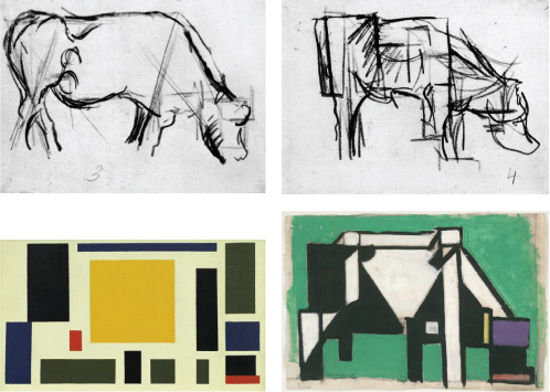
Figure 1: Theo van Doesburg: http://commons.wikimedia.org/ wiki/ File:Theo_van_doesburg_de_koe.jpg
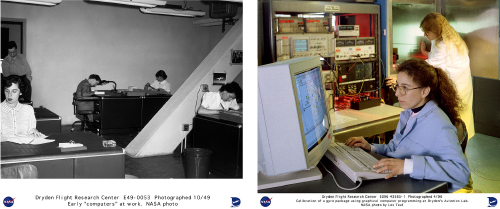
Figure 3a: NASA
Figure 3b: NASA
Figure 7: © ADAGP, Paris and DACS, London 2013
Figure 8: Professor Mark E. Bailey / Armagh Observatory
Figure 10: Courtesy of Dr David Goodchild
Figure 17: Courtesy of Tim Robinson
Videos of Jeannette Wing’s lecture in Section 3: © Florida Institute for Human & Machine Cognition (IHMC)
Every effort has been made to contact copyright owners. If any have been inadvertently overlooked, the publishers will be pleased to make the necessary arrangements at the first opportunity.
Don't miss out:
If reading this text has inspired you to learn more, you may be interested in joining the millions of people who discover our free learning resources and qualifications by visiting The Open University - www.open.edu/ openlearn/ free-courses