Economics and the 2008 crisis: a Keynesian view

Introduction

Decisions, decisions, decisions. Governments need to make decision about how much to spend, how to finance their debt and how much revenue to collect, in order to ensure their citizens’ welfare is as high as it can be, given that there is a limited amount of resources available or borrowable against future repayments. These decisions become even more pressing and their consequences more acute in times when the economy is not growing; or worse, in moments when it is actually shrinking. As the famous economist Paul Krugman wrote in 2012, 'times of crisis are when economists are most needed. If they cannot get their advice accepted in the clinch – or worse yet, if they have no useful advice to offer – the whole enterprise of economic scholarship has failed in its most essential duty'.

In this OpenLearn course you will work through seven sections in which you will engage with some of the major aspects of economic policy:

• What types of problems are governments concerned with?
• Which policy instruments do they have at their disposal?
• How do they make decisions about the effectiveness of alternative courses of action?

One of the most challenging aspects of economic policy and decision making is the study of how changes in economic variables influence the more immediate and the future economic response. As Charlie Bean, the deputy governor of the Bank of England in the early 2010s, puts it, 'people describe the steering of the economy like driving a car when all you can do is look through the rear view mirror'.

Figure 1

Show description|Hide description

This shows a boy on a ladder, spray painting graffiti on a wall. There is already writing on the wall which says, in large letters, ‘Running the economy’. The boy has sprayed out the first ‘n’ and has replaced it with an ‘i’ – changing it to ‘Ruining the economy’.

Figure 1

So, any claims as to what will happen in the future as a result of current policy are grounded in economic models about how economies, people, firms and industries within them, will respond. In this course you will discover that different economists have different theories about how the economy works, and different theories lead to different results, depending on the state of economies. This creates considerable controversy over which policies are right – you might already have your own views too.

You will also learn about the ways in which John Maynard Keynes’s theories revolutionised the thinking about how economic crises appear and how the government can solve them. In doing so, you will start to build an economic model to explore Keynes’s ideas.

Keynes’s thinking was very influential with economists and policymakers for several decades following the 1930s, but then fell out of favour for a time. The economic downturn that started in 2008 led to a widespread revival of interest as economic conditions seemed to resemble those seen in the 1930s. So a study of Keynes’s ideas is not just of historical interest but highly relevant to modern policymaking too.

This OpenLearn course is an adapted extract from the Open University course DD209 Running the economy.

Learning outcomes

After studying this course, you should be able to:

• understand what economists mean by ‘models’ and how they can be used to inform economic policy

• define the concept of equilibrium and explain how it can occur at low levels of output

• begin to understand the Keynesian model of aggregate demand and how it explains why economies can get stuck in a low output equilibrium

• critically evaluate the role of fiscal policy in changing the economy.

1 Keynes in context

Before we start to develop our Keynesian model of the economy, it is helpful to know something about Keynes and the context that compelled him to develop his theories, which are still influential today. Below you will find a timeline of some of the highlights in Keynes' life, and an audio clip in which two Open University economists discuss some key economic ideas, and Keynes' influence in shaping economics and economic policy.

Click on the link below to launch the timeline and then click and drag your mouse to move along the timeline for highlights in the life and career of John Maynard Keynes (1883–1946). Click on each entry to read some details.

Now listen to the following audio. This audio is taken from Block 2 of the Open University course DD209 Running the economy so there are a number of references to the block, as well as a summary of Block 1 of the course, which you should ignore. As you listen to the discussion, you may find it helpful to note down the key points.

Download this audio clip.Audio player: Open University economists discussing Keynes' ideas and influence

Show transcript|Hide transcript

Transcript: Open University economists discussing Keynes' ideas and influence

INTERVIEWER

I’m joined by Jonquil Lowe and Andrew Trigg who both teach Economics at The Open University. Both have been heavily involved in Block 2. So if we could start with you Jonquil, can you talk us through how Block 2 picks up from Block 1?

JONQUIL LOWE

Yes, Block 1 was all about data and how data can tell us something about the state of the economy and whether things are going wrong. That’s a bit like looking at the dashboard of a car. And just as with a car if you’re looking at the dashboard and the red lights are flashing you want to know what can policymakers do to steer the economy back on track. And that’s essentially what Block 2 is all about.

INTERVIEWER

But the economy is of course much more complex than a car, Andrew.

ANDREW TRIGG

Well yes there are different ideas about how an economy works. So we’re not sure whether the car’s the right analogy really but we’re going to run with it and see if we can try and introduce some basics of economics using that approach. One approach is that the economy is self-correcting. That there’s no need for government intervention. Until the 1920s that was the main approach followed in economics. There was a change then in the Great Depression with the unemployment and the crisis, the banking crash of 1929, where the great economist John Maynard Keynes came in and said we can do something; we can intervene to make a difference when there’s unemployment and crisis. The car analogy comes in there whereby, you know, we can steer the car. We can steer through economic problems.

JONQUIL LOWE

Well a bit more than that he actually said we have to steer the car, if we don’t steer the car, we’re on a collision course.

INTERVIEWER

And how influential were his ideas in those days?

ANDREW TRIGG

Well throughout the 1920s nobody was listening to him really. It was only in the 1930s when the Great Depression set in that his ideas were listened to. In 1936 his General Theory was published. And that had a huge impact internationally.

INTERVIEWER

And what were the ideas that he was advocating at that time?

ANDREW TRIGG

Well his main idea was that he used to joke that you should pay people to dig holes and fill them in again. And that that would get the economy going because if people were paid money then they would spend money and other people would be employed making things that would be consumed by the people who were being paid to dig the holes. Of course he thought the money would be spent on more important things, useful things.

INTERVIEWER

Shall we just talk about fiscal policy and monetary policy because a key for students in this block is understanding the difference between the two?

JONQUIL LOWE

Yes. Fiscal policy and monetary policy they’re both strands of what we call macroeconomics. And macroeconomics was really invented by Keynes. Before Keynes there was a very laissez-faire attitude towards the economy and a feeling that along with the teaching of Adam Smith, if you like, that if everybody pursued their own self-interest then collectively the economy would work and everybody would have jobs. And the Great Depression showed that that wasn’t the case. If individuals pursue their own self-interest sometimes the economy actually doesn’t work fine. It goes wrong. There simply aren’t enough jobs in the economy for people.

And so the two strands of policy to try and steer the economy and keep it operating towards the full employment level are fiscal policy and monetary policy. Now Keynes is very much associated with fiscal policy but in some respects that’s a bit misleading because he was also a monetarist. But fiscal policy is all about using government spending and taxation to put more money into the hands of the people who can go out and spend and get income circulating in the economy as a whole.

And Keynes said this was really important because sometimes the economy fails because the private sector loses confidence in the economy. Loses what he called animal spirits. And then firms hang on to their money. They don’t want to invest. The economy doesn’t grow. And it’s important in that situation for the government to step in and for the public sector to make the investment that the private sector won’t. So that’s fiscal policy. Monetary policy has become, at least until the financial crisis in 2008, the mainstay of just keeping the economy ticking over in non-crisis times. And this works more indirectly. If we’re going to thrash our car analogy then fiscal policy is a bit like putting your foot on the accelerator and sometimes on the brake. Whereas monetary policy is rather more like driving through the gears. It’s more indirect.

So conventionally it involves using the interest rate. So if interest rates are low then it’s cheap for firms to borrow, that tends to stimulate investment. It’s also as you know, if you have a mortgage say, if interest rates are low then you can borrow to buy a big house. The housing market, as it booms you feel wealthy. You feel more confident. You go out and spend and that all helps the economy as well. So interest rates can be raised and lowered to influence the level of activity in the economy. And that’s the essence of conventional monetary policy.

INTERVIEWER

Andrew, how important is it for students to really have a clear idea of what the difference is between monetary and fiscal policy?

ANDREW TRIGG

Well they're the main policy choices for the government and for the Bank of England, the government in the UK, traditionally it’s the Treasury Department that decides fiscal policy. So that involves its spending decisions: how much to spend on the National Health Service, how much to raise in terms of taxes, setting VAT and so on and so forth. Monetary policy is decided in recent years by the Bank of England. The Bank of England sets the rate of interest. And does other things as well which this block talks about, in terms of how much money it releases into the financial system. So it’s important what interest rate policy, monetary policy is and it’s important what spending and taxation policies. Those are big decisions for macroeconomics, for running the economy as a whole. And they have international implications in terms of how much money flows into the economy, exports and imports.

INTERVIEWER

So how do policymakers know how much accelerator to apply to use your car analogy or which gear to choose?

JONQUIL LOWE

That’s where economic models come in and building an economic model is going to be a core activity in this block. So using an economic model is a bit like lifting the bonnet and looking at how the engine works. An economic model is a representation or an image of the economy that focuses on the key factors, the key relationships in the economy.

ANDREW TRIGG

And it relates back to what we were saying about the dashboard of the car in terms of the information about the car, the temperature gauge and so on and so forth. That with the economy we’ll be looking at the level of output GDP, which we’ve looked at in Block 1, we’ll be looking at the level of inflation and unemployment, and this block we’ll focus mainly on unemployment and GDP. So driving the car you’d be looking at these indicators, you'd be steering the economy. And the model would help to look at the gearstick, the accelerator pedal, how you try and react to these indicators.

INTERVIEWER

So clearly sometimes it works and sometimes it doesn’t. And when we had the financial crisis in 2008, did the model break down?

ANDREW TRIGG

Well the Queen asked the question why did nobody predict this? Why did nobody see this crisis? It did provoke a major change of thinking in economics about whether we have really understood how economies work. We had a period of boom. Gordon Brown told us that boom and bust was over. We had this period of growth throughout the 1990s and into the 2000s. And then there was this major, as we all know, financial crisis that started in 2007. You might call it an epic recession that started in 2008. Suddenly Keynes was back. There was a return of Keynes. He’d been sort of forgotten about during the post-war period. And suddenly Chancellors throughout the world, finance ministers, were discovering Keynesian levers on how to react. Even though the borrowing was going up, governments were spending more than they were earning. The governments were spending money in a Keynesian approach to try and get the economy out of the crisis to reduce the borrowing because of all the money that’s been spent on unemployment benefit. All the waste involved with high unemployment, governments were spending. This was the Keynesian response, macroeconomic response to the recent economic crisis of 2008.

End transcript: Open University economists discussing Keynes' ideas and influence

Download

Open University economists discussing Keynes' ideas and influence

2 Planned and actual values

The economy as modelled by the circular flow diagram, below, appears to be a rather peaceful place, where expenditure is always identical to output and saving is always identical to investment. But saving decisions and investment decisions are made by different people, so it seems there is no reason why they should match, and Keynes’s model of change in national income depends precisely on expenditure being too great or too small to match output and hence on saving being too small or too great to match investment.

Figure 2 Circular flow of income

Show description|Hide description

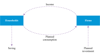
Flows of money are shown by dashed lines with directional arrowheads.

A flow labelled ‘Income’ runs from Firms to Households.

A flow labelled ‘Planned Consumption’ runs from Households to Firms.

A dashed line pointing vertically down from Households is labelled ‘Saving’.

A dashed line pointing vertically up to Firms is labelled ‘Planned Investment’.

Figure 2 Circular flow of income

Activity 2

Watch the video below to see how this paradox is resolved. This video is part of the Open University course DD209, Running the economy, so there will be references to Block 1 of the course, which you should ignore.

Download this video clip.Video player: Planned and actual values

Show transcript|Hide transcript

Transcript: Planned and actual values

NARRATOR

The familiar circular flow diagram shows the flows of incomes, consumer expenditure, saving and investment. Suppose households decide to save more and, therefore, to consume less. How can it be that investment automatically increases to compensate?

As households spend less in the shops, firms will find that their stocks of unsold consumer goods will build up. This counts in the national income accounts as additional investment, although it is unplanned. The identity – saving equals investment – still holds but only because of the way in which the terms 'saving' and 'investment' are defined for accounting purposes.

Now for the opposite story. Suppose households decide to save less and, therefore, to consume more. One possible outcome is that firms will run down stocks to satisfy the extra demand. This counts as unplanned disinvestment, so the lower saving is accommodated by reduced investment.

But suppose firms have no spare stocks to run down. How can saving still equal investment? Think about this before continuing with the tutorial. [PAUSE] The answer is that if firms have no spare stocks, households' plans to save less and consume more will be frustrated since there is no more available to buy. Part of their saving will now be unplanned, but neither total saving nor total investment will change.

The national income identities you studied in Block 1 belong to the world of the accountant in which every change in a variable is compensated by a corresponding change in another, so that the accounts always balance. The national accounts record the values of actual expenditure and actual output. So an increase in stocks – called inventories in the national accounts – even if unplanned, is recorded as investment. And unplanned saving by households is reflected in the recorded level of consumption.

But none of this means that planned expenditure will always equal output or that planned saving will always equal planned investment. And if plans don't accord, then, as we have seen, someone's plan will be thwarted. We consider now what happens to national income when plans do not accord. We will start by reinterpreting the circular flow diagram.

The diagram is familiar but, now, the labels are going to mean something rather different. Consumer expenditure now means planned consumer expenditure. This is how much households would like to spend given the income that they have. So saving now means how much they would like to save – planned saving. And investment now means how much firms would like to invest – planned investment.

Let's start off with these plans in harmony so nothing is rocking the boat. But now, suppose that households spontaneously decide to consume more. The flow of consumption expenditure becomes stronger as they save less. But this doesn't mean firms simultaneously plan to invest less. So there is a surge of expenditure, and the boat does rock.

The balance of the economy has been upset, or to put it another way, the equilibrium has been disturbed. Recall that, in equilibrium, there is no impetus within the model for any economic agents to change their behaviour. Households are not coming under pressure from changed incomes to change their consumption or saving plans. And firms are not coming under pressure from changed demand to change their production plans.

Following the spontaneous surge of consumer spending, however, there is an impetus for firms to change their behaviour by producing more to satisfy the extra demand. Equilibrium is quite different from identity. Actual saving and actual investment will still be identical when households increase their spending, as stocks will be run down, but the equilibrium equality between planned saving and planned investment will no longer hold true.

If firms do not wish to see their stocks depleted for long, they will need to increase production. According to Keynes's theory, this imbalance will put in train a process that will lead to a restoration of equilibrium. National income will increase as firms respond to the extra consumption demand by producing more, and therefore, paying out more in incomes. And equilibrium will be restored at a higher level of income when the additional income earned is sufficient to increase planned saving to its previous level.

End transcript: Planned and actual values

Download

Planned and actual values

Interactive feature not available in single page view (see it in standard view).

Active content not displayed. This content requires JavaScript to be enabled.

Interactive feature not available in single page view (see it in standard view).

3 The consumption function

So far, we have been representing what happens in the economy using the circular flow of income model.

To demonstrate Keynes’s theories about equilibrium in a more quantifiable way, we need to use what is called the aggregate demand model. The two main components of this model are consumption and investment. Section 6 will show you an extended version of this model which includes government expenditure, but for now, Figure 3 represents an economy with no government and no trade and relations with other countries. This section consolidates your understanding of the first element in this model: the consumption function.

Figure 3 The aggregate demand model

Show description|Hide description

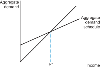
The diagram shows an aggregate demand schedule.

The diagram contains a vertical axis, which is labelled as ‘Aggregate Demand’ and a horizontal axis which is labelled as ‘Income’.

There is a straight line from the origin, sloping upwards at 45 degrees.

The aggregate demand schedule is a straight line, sloping up from left to right, from a point about one quarter of the way up the vertical aggregate demand axis. The slope of the schedule is quite shallow.

The aggregate demand schedule intersects the 45 degree line about half way along the 45 degree line. From this point of intersection, a dashed vertical line is taken down to the horizontal Income axis, to a point on the axis labelled as capital letter Y followed by a star.

Figure 3 The aggregate demand model

3.1 Building a consumption function (1)

According to Keynes, there is a fairly stable relationship between planned consumption and current income. Households plan to spend a fairly constant proportion of each additional pound they earn. He calls this proportion the ‘marginal propensity to consume’. To present this diagrammatically, we start with two axes at right-angles to each other.

3.2 Building a consumption function (2)

We now have a hypothetical consumption function.

3.3 Building a consumption function (3)

Activity 5

Look at Figure 6 and answer the following question.

Figure 6 A more realistic consumption function

Show description|Hide description

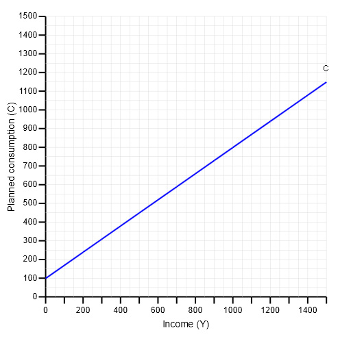
The diagram shows a consumption function, labelled as C.

The vertical axis is labelled as ‘Planned consumption (C))’ and has values from 0 to 1500, at intervals of 100. The horizontal axis is labelled as ‘Income (Y)’ and has values from 0 to 1500, at intervals of 100.

The consumption function is a straight line that slopes upwards, starting from point 100 on the vertical axis. The upward slope is fairly steep but less than 45 degrees. The end point of the function on the diagram is at Y of 1500 and C of 1150. Coordinates of points the consumption function passes through include, for example, (500Y,450C) and (1000Y, 800C).

Figure 6 A more realistic consumption function

What is the equation of this revised consumption function?

To use this interactive functionality a free OU account is required. Sign in or register.

Interactive feature not available in single page view (see it in standard view).

Answer

The equation is: C = 100 + 0.7Y

4 Modelling equilibrium

We have said that the economy will be in equilibrium when planned saving matches planned investment. So we need to use our diagram to explore this relationship. First, we need to show planned saving. Our diagram already shows planned consumption at each level of income, and of course planned saving is simply the difference between income and planned consumption. Having shown saving, we need to go on to add investment to our model to complete our analysis of equilibrium.

4.1 Modelling planned saving (1)

A good way to make our diagram work for us to show planned saving (the difference between income and planned consumption) is to start by reflecting each value of income plotted on the horizontal axis on to the vertical axis where planned consumption is plotted. This will make it easy to compare visually each level of income with its corresponding level of planned consumption. So let’s start with just the two scaled axes and imagine that each value of income emits a ray of light vertically. A mirror is held diagonally to reflect that ray on to the vertical axis. Click on each circle on the bar underneath the chart, working from left to right to watch this process build up step by step.

The line we have traced out is called, for obvious reasons, the 45-degree line, and it shows us at a glance how far up from the horizontal axis any value of income would appear if we plotted it on the vertical axis. At any point on the line, the variable plotted on the vertical axis – planned consumption – is equal to the variable plotted on the horizontal axis – income.

4.2 Modelling planned saving (2)

If we now show our consumption function on the same diagram, we can visually compare each level of income with its corresponding level of planned consumption.

4.3 Modelling planned investment

At an income level of £600, households are planning to spend £520 on consumption and to save the remaining £80. But firms are not planning to invest at all! Let’s now incorporate planned investment into our diagram. This will mean two slight changes.

1. We re-label the vertical axis ‘Aggregate demand’, as we are adding investment demand to consumption demand.
2. We reinterpret the 45 degree line accordingly. Recall that at any point on the 45-degree line the variable plotted on the vertical axis is equal to the variable plotted on the horizontal axis. So in this diagram, at any point on the line, aggregate demand is equal to income.

The Keynesian model treats planned investment as an exogenous component of demand, that is, as not dependent on current income. It will therefore appear as a horizontal line on our diagram but, when we add planned investment to planned consumption, the aggregate demand line, which at present shows only planned consumption, will move upwards by the amount of planned investment we introduce.

4.4 And so to equilibrium

In our diagram, planned saving is shown by the vertical gap between the consumption function and the 45-degree line. Planned investment is shown by the vertical gap between the consumption function and the aggregate demand function.

Given the assumptions we have made about exogenous consumption, the propensity to consume and the level of exogenously determined investment, these two vertical gaps are equal at an income level of £600, so at this income level planned saving = planned investment. We have therefore illustrated an economy in equilibrium at an income level of £600.

Note that the AD line (C + I) crosses the 45-degree line at an income level of £600. Since at any point on the 45-degree line AD = Y, we can say that at an income level of £600 aggregate demand = income.

Figure 10 Equilibrium at an income level of £600

Show description|Hide description

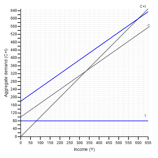
The diagram shows an aggregate demand (C+I) function, a consumption function (C), a planned investment function (I) and a 45 degree line.

The vertical axis is labelled as ‘Aggregate Demand (C+I)’ and is marked from 0 to 640, at intervals of 40. The horizontal axis is labelled as ‘Income (Y)’ and is marked from 0 to 650, at intervals of 50.

The 45 degree line slopes up from the origin.

The planned investment line (I) is horizontal, drawn across from the point 80 point on the vertical aggregate demand (C+I) axis.

The consumption function (C) slopes upward more shallowly than the 45 degree line, from the point 100 on the vertical axis.

The Aggregate Demand function (C+I) is in shown in blue and lies above and is parallel to the consumption function (C). It slopes upward from the 180 point on the vertical axis. The vertical gap between the C+I and the C function is equal to the value of planned investment (I).

The Aggregate Demand (C+I) function intersects the 45 degree line at an income level of 600. At this point, Aggregate Demand also equals 600.

Figure 10 Equilibrium at an income level of £600

So we have two ways of looking at equilibrium in this simple economy.

When the economy is in equilibrium:

1. Planned saving = Planned investment
2. Aggregate demand = Income

5 When equilibrium is not enough

Keynes believed that an economy may settle into equilibrium at a level of income too low to support full employment.

We can use our model to illustrate this possibility and to illustrate how policy intervention to stimulate aggregate demand may bring about full employment.

5.1 Underemployment equilibrium

Equilibrium occurs when aggregate demand equals income, so, in the previous activity, when AD is equal to income at £600. But it may be that AD of £800 equal to Yf is needed to support full employment, so equilibrium would need to occur at an income level of £800. Given current consumption and investment habits, however, if income stood at £800, AD would be less than £800, as we can see from the fact that the C + I line lies beneath the 45-degree line at an income of £800. To achieve full employment, a policy intervention would be needed to stimulate demand sufficiently to bring about equilibrium at an income level of £800.

You will now use an Aggregate Demand tool to explore how we could move the economy to a full employment equilibrium.

Activity 8

Select the link below to access the tool.

Aggregate Demand tool

Place yourself in the tab 'Closed economy without government'. This means the economy has no government, and demand comprises only consumption and investment. Complete the following tasks.

Task A

(a) Set the inputs to the following values: exogenous consumption (labelled 'Consumption intercept' equals 100, the marginal propensity to consume is 0.7, investment is set at 80 and full-employment income is 800.

Answer

The outputs and chart in the tool should look like this. You can see that this economy is currently in equilibrium at an income of 600 but we want to reach the full-employment equilibrium of 800.

Maximise

Figure 11

Show description|Hide description

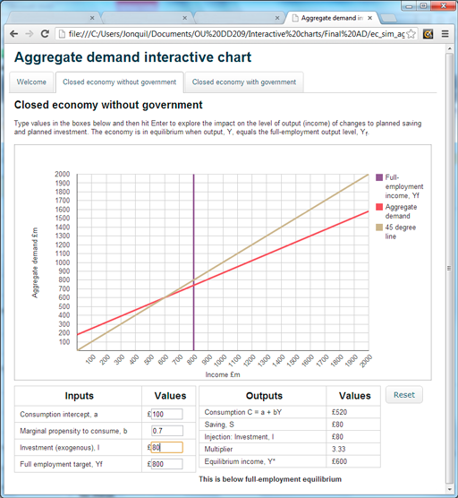
The figure is a screenshot of the Aggregate Demand Interactive chart.

It shows the answer to Activity 8 question (a) which asks you to input specified values for exogenous consumption, the marginal propensity to consume, investment and the full employment equilibrium.

The diagram shows what the Aggregate demand chart should look like with these values inputted. Above the chart, it says that this is for a closed economy without government.

Aggregate Demand in millions of £ (£m) is shown on the vertical axis, starting at 0 and rising to 2000, at intervals of 100. Income in £m is on the horizontal axis, starting at 0 and rising to 2000 at intervals of 100.

The 45 degree line is shown in brown. The Aggregate Demand function is shown in red. The full employment equilibrium level is shown at a level of income of £800m. A vertical full employment income line is drawn in purple from this point to intersect the 45 degree line.

Just on the right of the chart is a legend showing the colour coding for the three lines. This legend tells us that the full employment income is denoted as Yf.

The AD line intersects the 45 degree line at an income level Y of £600m, below the full employment level of income Yf.

Figure 11

Task B

(b) State by how much AD falls short of the level required to produce the full-employment income of £800.

To use this interactive functionality a free OU account is required. Sign in or register.

Interactive feature not available in single page view (see it in standard view).

Answer

In this example, aggregate demand at any level of income is calculated using the equation:

AD = 180 + 0.7Y

So, if equilibrium income (Y) were to be £800:

AD = 180 + 0.7 x 800 = 180 + 560 = 740

which would fall short of income by £800 – £740 = £60.

Policy intervention will be needed to give a stimulus that initially raises aggregate demand by £60.

Task C

(c) Assume that the required stimulus is going to take the form of policy to increase investment. Use the tool to change investment by the amount you calculated in (b).

Answer

If you increased investment by 60, the new amount of investment should be 140. The outputs and chart from the tool should now look like this:

Maximise

Figure 12

Show description|Hide description

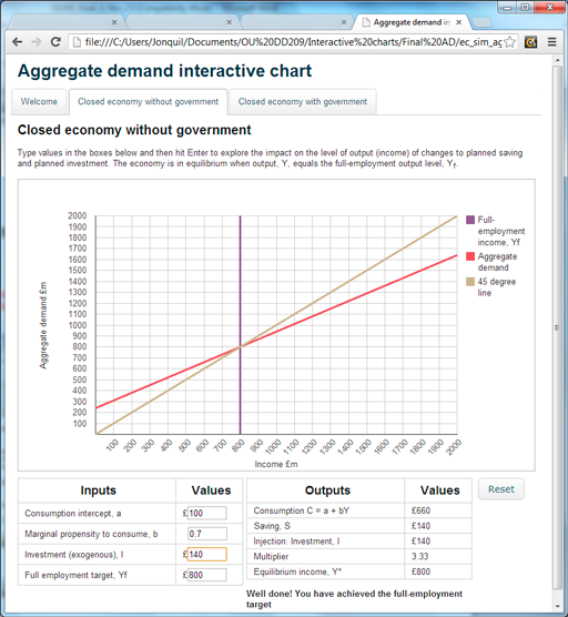
The figure is a screenshot of the Aggregate Demand Interactive chart.

It shows the answer to Activity 8 question (c). Above the chart, it says that this is for a closed economy without government.

Aggregate Demand in millions of £ (£m) is shown on the vertical axis, starting at 0 up to 2000, at intervals of 100. Income in £m is on the horizontal axis, starting at 0 and rising to 2000 at intervals of 100.

The 45 degree line is shown in brown. The Aggregate Demand function is shown in red. The full employment equilibrium level is shown at a level of income of £800m. A vertical full employment income line in purple is drawn from this point to intersect the 45 degree line. The legend on the right of the chart shows the colour coding for the lines and tells us that full employment income is denoted as Yf.

The AD line intersects the 45 degree line at an income level Y of £800m, which equals the full employment level of income Yf.

Figure 12

Task D

(d) Describe what has happened to the equilibrium level of income as a result of the change you made in (c).

To use this interactive functionality a free OU account is required. Sign in or register.

Interactive feature not available in single page view (see it in standard view).

Answer

The economy is now in equilibrium at an income of £800 which is the full-employment level of income.

6 The aggregate demand model with government and fiscal policy

The previous sections introduced some of the arguments made by Keynes as to why capitalist economies can become stuck in positions of high unemployment. Though there may be a quite stable relationship between income and consumption, private investment can languish at levels that are insufficient for full employment. The government may choose to fill the gap: an active state sector for Keynes can iron out the vagaries of volatile private investment spending. For the macroeconomy, the key problem is the failure to reach full employment owing to a shortfall in aggregate demand, and the component of aggregate demand that is most frequently insufficient is investment demand.

This section introduces some of the policy tools that are available to a government department responsible for coordinating public finance – in the UK called Her Majesty’s (HM) Treasury. The Treasury is the coordinating body that allocates government spending (for transport, health, education, defence, and so on) and oversees the collection of taxes (such as Income Tax, Value Added Tax (VAT) and excise duty on petrol). When the government uses these spending and revenue raising activities to stabilise the economy, this comes under the purview of fiscal policy, which is the main focus of this section.

It should be emphasised that the role of fiscal policy is highly contested by economists and policymakers. From a Keynesian perspective, the government has a vital role in stabilising the macroeconomy, because there is no automatic mechanism through which the economy can recover from a recession. For critics of the Keynesian approach, however, the government should leave the private sector alone: it is government intervention that prevents the private sector from bringing about full employment equilibrium. The purpose of this section is to introduce and explore the Keynesian point of view. Some critiques of the Keynesian approach are also explored.

Section 6 introduces government expenditure and shows its full potential Keynesian impact. Not only can government spending generate demand for goods and services that may encourage firms to employ more people, but also its effect on income can be much greater than the initial stimulus. The section then focuses on the more tricky issue of how government spending is financed through taxation. It also considers how the cutting of taxes can help to stimulate aggregate demand. These two dimensions of fiscal policy are brought together in a consideration of fiscal stabilisers. The government can use fiscal policy in a discretionary way to actively intervene in times of crisis; it can also allow what are known as automatic stabilisers to smooth out economic fluctuations. Finally, the section examines a big policy issue that has dominated public policy-making in recent years – the issue of budget deficits.

6.1 Government expenditure (1)

In modern capitalist economies, the public sector plays a key role. In the UK, total government expenditure was forecast to be £683 billion in the financial year 2012–13, which is 43.4% of Gross Domestic Product (GDP) (HM Treasury, 2012). Government activities range across all spheres of the economy, from the provision of social protection (such as benefits and pensions) to health, transport and defence. A breakdown of government spending is provided in Figure 13. Social protection is clearly the largest category, with health and education the next largest categories.

(Source: HM Treasury, 2012, p. 1, Chart 1)

Figure 13 UK government spending, 2012–13 (£ billion)

Show description|Hide description

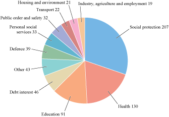
This diagram is a pie chart, divided into eleven sections showing the breakdown of government spending. The data source is HM Treasury, 2012, page 1, chart 1.

The largest category is Social protection, at £207bn.

Then, moving clockwise the pie chart presents the other categories of spending in descending order:

Health 130; Education 91; Debt interest 46; Other 43; Defence 39; Personal social services 33; Public order and safety 32; Transport 22; Housing and environment 21; Industry, agriculture and employment 19.

Figure 13 UK government spending, 2012–13 (£ billion)

Social protection includes the provision of transfer payments, where there is a transfer from the government to individuals that is not made in return for any services. Old-age pensions and unemployment benefit are examples of transfer payments. If, for example, a refuse collector becomes unemployed and receives unemployment benefit, this benefit is a transfer payment, since he is providing no direct service. By contrast, if the refuse collector is in work and paid a wage by the government, that is government spending on the service of emptying bins.

As you will see in the analysis that follows, some economists and policymakers may regard government expenditure as unproductive and wasteful, a drain on the wealth-creating private sector, even when it takes the form of expenditure on goods and services. For Keynes, however, government expenditure represents a powerful lever for intervention when the private sector fails to generate sufficient demand.

Keynes formulated his ideas during the 1920s, making a number of attempts to persuade the UK government to increase its expenditure in order to boost aggregate demand. Although the wartime British Prime Minister, David Lloyd George, had promised that there would be ‘jobs for the boys’ when soldiers came home after the First World War, this did not materialise. High unemployment in the 1920s led to the decline of the Liberal Party, of which Lloyd George was the leader, and its replacement by James Ramsay MacDonald’s Labour Party as the main alternative to the Conservatives – a position from which the Liberal Party (calling itself the Liberal Democrats at the time of writing) has never recovered.

In one final push, in the 1929 General Election, Lloyd George tried to regain his supremacy over the ‘spectre’ of socialism. Under his auspices, the Liberal Party published a pamphlet entitled ‘We can conquer unemployment’. He also marshalled the support of Keynes to develop his party’s manifesto. In his address to Liberal candidates on 1 March 1929, Lloyd George pledged: ‘If the nation entrusts the Liberal Party at the next General Election with the responsibilities of government, we are ready with schemes of work which we can put immediately into operation, work of a kind which is not merely useful in itself but essential to the well-being of the nation’ (Keynes, 1972, p. 88).

The Conservative-dominated press rubbished these claims as the fantasies of a Welsh windbag, being far too optimistic and not based on common sense. Keynes piled in, in a pamphlet entitled ‘Can Lloyd George do it?’, written with a politician, Hubert Henderson. This aimed to supplement and to answer criticisms of the Liberal Party pamphlet mentioned above. Keynes wrote:

In answer to the objections raised by the then Conservative Prime Minister Stanley Baldwin, Keynes observed: ‘Mr Baldwin and his colleagues are not more capable of expounding the true economic science of the matter than they would be of explaining to you the latest propositions of Einstein’ (Keynes, 1972, p. 91).

6.2 Government expenditure (2)

Lloyd George’s £300 million programme had three main planks:

• Transport: To modernise the rail and transport system, including electrification of railways and particular emphasis on roads, since they were under the direct control of the government sector. A capital sum of £145 million for road replacement and extension over two years was proposed.
• Housing: To build 200 000 houses a year: a million houses over a ten-year period would provide for slum clearance and reduction of overcrowding. Unemployed building workers would be set to work on these road- and house-building programmes.
• Small projects: A host of other small developments, such as telephone development and land drainage. All this required was a Treasury green light for ‘innumerable schemes pigeonholed in government offices’ (Keynes, 1972, p. 99).

Similar public spending programmes were announced throughout the world in response to the economic crisis of 2008. In the USA, President Obama introduced the American Recovery and Reinvestment Act of 2009, which resulted in US$831 billion of government spending on items such as infrastructure, health and education. In the same year, Australia launched a ‘Nation Building and Jobs Plan’, costing AUS$42 billion, on items such as building local community infrastructure and refurbishing schools – estimated to create 90 000 jobs and to boost annual GDP by 1% after two years (Vu and Tanton, 2010, p. 129).

The official UK government position in 1929, however, as summarised by the Balfour Committee on Industry and Trade, was that a programme of this kind ‘could not provide employment in their own trades for any considerable number of unemployed persons’ (quoted in Keynes, 1972, p. 100). Against this pessimistic assessment, Keynes stated the Liberal position that ‘each million pounds spent annually on road improvements would employ, directly or indirectly, 5,000 workpeople’ (Keynes, 1972, p. 103). Keynes pointed out that this is four times higher than the assessment given by the Balfour Committee. The committee had failed to take into account the indirect employment effects of the road-building programme.

This error was eventually admitted, after questioning in the House of Commons, by the Conservative Minister of Transport, Colonel Ashley. After noting that for each £1 million of road-building expenditure employment ‘might be increased to as much as 2,500’, Colonel Ashley conceded that for each of these direct jobs ‘another man would be indirectly employed in producing and transporting materials in other ways, and this assumption may not be unreasonable’ (quoted in Keynes, 1972, p. 104). There would be additional indirect employment created in the production and transport of the tarmac and other materials that are required for road-building, leading to a further possible 2500 jobs.

In Keynes’s view the Balfour Committee had failed to take account of something much more significant than the indirect employment to which the Liberal Party’s pamphlet and statements had drawn attention. By putting unemployed people into work both directly and indirectly, an initiative such as the road-building programme would increase what he called ‘effective purchasing power’. Newly employed workers in the road-building industry would spend part of their wages on a wide range of goods and services, providing increased income and creating further new jobs in other parts of the economy. This in its turn would lead to further spending, more income and more new jobs. In this way there would develop a considerable ripple in the form of successive rounds of spending: ‘the forces of prosperity [would] work with a cumulative effect’ (Keynes, 1972, p. 106).

This notion of cumulative increases in demand and hence in income and output is so central to Keynes’s system that it is worth quoting at some length from the pamphlet that he wrote with Henderson:

By the time Keynes published The General Theory of Employment, Interest and Money in 1936, he had refined his thinking about these cumulative effects and showed how they might be estimated using the marginal propensity to consume.

The analysis that follows in the next section shows how the impact of government expenditure on output and employment can be modelled, using the aggregate demand framework.

6.3 Government expenditure (3)

To model the impact of government expenditure, the first step is to introduce a new term G to represent planned government spending. Whereas earlier it was assumed that the economy consisted only of private agents (households and firms), the government sector (also called the public sector) is now included in the model. Like private investment, government spending is treated in this model as exogenous.

It is important to note that the portion of government spending that takes the form of transfer payments is not included in G since it adds nothing directly to the demand for goods and services. However, as you will see, transfer payments do affect the household consumption component of aggregate demand and income.

Aggregate demand (AD) in the extended model consists of planned consumption (C ) and planned investment (I ), as before, with an additional term (G ) representing planned government spending:

AD = C + I + G

Some elements of spending may form part of I at one time in history and part of G at another. For example, investment in railways in the 1920s would be categorised as part of private investment (I ), whereas after railway nationalisation in the 1940s such investment would be categorised as part of government spending (G ). Keynes made the point that expenditure by the government on roads was equivalent to private investment in the railways. In fact, since in times of stagnation, the private sector might be reluctant to invest, government spending can be required to fill the gap – not just to boost aggregate demand, but also to provide vitally needed infrastructure investment.

This new role for government spending can now be shown in the aggregate demand diagram (Figure 14). In this diagram, government spending (G ) and investment (I ) are shown as exogenous elements of aggregate demand, unaffected by changes in income. The combined total of government spending and private investment (I + G ) is represented by a horizontal line. Also exogenous is the intercept of the consumption function (a). You may recall from earlier sections that the slope of the consumption function is represented by the coefficient b.

Figure 14 Government spending and aggregate demand

Show description|Hide description

This diagram has Aggregate Demand (AD) on the vertical axis and Income (Y) on the horizontal axis.

A solid line at a 45 degree angle is drawn upwards from the origin.

From a short way up the vertical axis, a horizontal line is drawn. This is labelled I+G.

A little above this horizontal line, from point ‘a’ on the vertical axis, a straight line is drawn upwards, with a shallower slope than the 45 degree line. This is labelled ‘Consumption function, C=a+bY.’

Somewhat above the consumption function, and parallel to it, is a line drawn from a point on the vertical axis a+I+G. This line is labelled ‘Aggregate Demand schedule, AD=C+I+G.’

Figure 14 Government spending and aggregate demand

To derive the new aggregate demand schedule, the horizontal line for combined investment and government spending can be added to the consumption function. The new aggregate demand schedule AD = C + I + G has an intercept a + I + G and the same slope (b) as the consumption function.

6.4 Government expenditure (4)

The aggregate demand model can also be used to illustrate what might happen under an increase in government spending, as shown in Figure 15. Let government spending increase by £300 million – money that could be spent along the lines of the 2009 Obama Recovery Act or the 1929 Lloyd George three-point plan. This is shown by an upward shift of the intercept of the aggregate demand schedule by £300 million due to an increase in government spending from G₀ to G₁. It is referred to in modern economics as a fiscal stimulus. Using one of its key fiscal powers – the ability to carry out expenditure – the government is able to boost aggregate demand.

Figure 15 Modelling a fiscal stimulus

Show description|Hide description

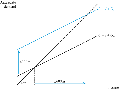
This diagram has Aggregate Demand (AD) on the vertical axis and Income (Y) on the horizontal axis.

A solid line at a 45 degree angle is drawn upwards from the origin.

From a short way up the vertical axis, a straight line is drawn, sloping upwards at an angle shallower than 45 degrees. This line is labelled as C+I+G zero and it intersects the 45 degree line quite low down. A dashed line is drawn from this intersection point down to the horizontal Income axis.

From a point about half way up the vertical axis, a second straight line is drawn. This is parallel to the first one and is labelled as C+I+G1. This intersects the 45 degree line much further along. A dashed line is drawn from this intersection point down to the horizontal Income axis. This point is much further along the axis than the point from the first aggregate demand schedule.

There are two arrows in blue showing the direction of change. One arrow points upward along the vertical axis, from the lower to the higher aggregate demand schedule. This has £300m written beside it.

Another arrow runs to the right along the horizontal axis, from the lower point on the axis to the higher point. This has £600m written beside it.

Figure 15 Modelling a fiscal stimulus

This ‘double your money’ insight can now be explained by breaking down the effect of the stimulus into a series of rounds, as shown in Table 1. In Round 1, the change in income is equal to the fiscal stimulus of £300 million. Round 2 then depends on how much of this income is spent.

It is modestly assumed in Figure 15 that the marginal propensity to consume – the slope (b) of the consumption function – is equal to 1/2. This means that in Round 2, half of the initial increase in income from the fiscal stimulus will be spent on consumption, as shown by the £150 million change in income. By Round 2 it therefore follows that there is a cumulative increase in income of (i) the initial direct increase in income of £300 million, and (ii) the additional indirect impact of £150 million. These two items add up to a cumulative income of £450 million in Round 2.

This process continues in Round 3, with half of the previous round’s change in income (£150 million) spent as consumption: a new change in income of £75 million. In each round, half of the previous round’s change in income is spent; these rounds continue indefinitely. By Round 10, however, the change in income has fallen to just over half a million pounds, and the cumulative change approaches its final value of £600 million – the doubling of income that is illustrated in Figure 15. Even by Round 3, 87.5% of the eventual cumulative change in income has occurred, so although in theory the expansionary effect may take many rounds and a great deal of time to work itself out, the main impact is felt quite quickly.

Figure 16 shows the first three rounds. In Round 1, the injection of government demand leads to an upward shift of the aggregate demand schedule by £300 million. Initially, this planned aggregate demand exceeds current output. At the outset, in Round 1, only £200 million worth of output (income) is being produced, yet now the total aggregate demand is £500 million. If the key assumption is now made that there is sufficient spare capacity – idle factories or machinery, and a pool of unemployed workers – then in response to the additional demand, output can be increased by £300 million, as depicted by the first horizontal arrow.

Figure 16 Direct and indirect impacts of a fiscal stimulus

Show description|Hide description

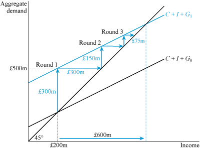
This diagram has Aggregate Demand (AD) on the vertical axis and Income (Y) on the horizontal axis.

A solid line at a 45 degree angle is drawn upwards from the origin.

From a short way up the vertical axis, a straight line aggregate demand schedule is drawn, sloping upwards. This is labelled as C+I+G zero. This has a shallower slope than the 45 degree line and intersects the 45 degree line quite low down. A dashed line is drawn from this intersection point vertically down to the £200m point on horizontal Income axis.

From about half way up the vertical axis, a second aggregate demand schedule is drawn. This is parallel to the first one. This is labelled as C+I+G1. This intersects the 45 degree line much further along the line. A dashed line is drawn from this intersection point down to the horizontal Income axis. This point is much further along the axis than the point from the first aggregate demand schedule.

The diagram shows three rounds of the fiscal stimulus process, via a series of vertical and horizontal arrows that form three steps. The arrows decrease in length as we move from left to right.

The first vertical arrow runs from the point of intersection between the lower aggregate demand schedule and the 45 degree line directly up to the higher aggregate demand schedule. This has ‘£300m’ written beside it. . Above the point where the arrow hits the higher aggregate demand schedule is written ‘Round 1’.

From the point where the vertical arrow hits the higher aggregate demand schedule, an arrow runs horizontally right to hit the 45 degree line. This arrow has ‘£300m’ written beside it. Another arrow runs vertically up from this point on the 45 degree line up to the higher aggregate demand schedule, with ‘£150m’ written beside it. Above this point is written ‘Round 2’.

From this point on the higher aggregate demand schedule an arrow runs horizontally right to the 45 degree line, and then vertically up to the higher aggregate demand schedule. This has ‘£75m’ written beside it and above is written ‘Round 3’. A final short arrow is drawn horizontally to the 45 degree line. This is just short of the equilibrium position, where the higher aggregate demand schedule intersects the 45 degree line.

There is one further line on the diagram. From the point where the first vertical arrow hits the higher aggregate demand schedule, a dashed line is taken horizontally left to the vertical axis, to a point labelled ‘£500m’

Figure 16 Direct and indirect impacts of a fiscal stimulus

In Round 2, the new stimulus of £150 million, as shown in Table 1, comes into play. Once again aggregate demand exceeds current output, this time by £150 million, and a new horizontal line indicates the increase in output to match this demand. Similarly, in Round 3 the impact of the £75 million boost in aggregate demand is matched by a £75 million boost in output. These rounds eventually peter out, as in Table 1, when both aggregate demand and aggregate output have increased by £600 million.

The process, illustrated in Table 1 and in Figure 16 is referred to by Keynes as the multiplier process, since the impact of the fiscal stimulus is multiplied throughout the economy. The multiplier captures the cumulative effect of a change in spending on income. The change represented here is a change in government spending, but the model could also be used to show the effect of a change in another exogenous factor such as investment.

Let Δ denote the amount by which a variable might change. The multiplier can be expressed in mathematical terms as the ratio of the eventual change in income (ΔY ) to the initial change in spending that caused it (ΔG ):

The size of the multiplier depends on the marginal propensity to consume, as explored in the box below. It has a simple formula:

where b is the marginal propensity to consume. In the example in Table 1, the propensity to consume is equal to 1/2. Hence

The eventual doubling of income in the multiplier process is captured in total by this formula for the multiplier.

Since the concept of the multiplier emerged in the 1930s, economists have used statistical methods to estimate its empirical size. There is, however, considerable uncertainty as to the multiplier’s precise value. At the top end of estimates of the size of the multiplier, Eggertsson (2006) finds the multiplier to be as high as 3.8. In a more recent survey, Ramey (2011) pronounces that the ‘range of plausible estimates for the multiplier … is probably 0.8 to 1.5’. Due to the uncertainty involved, however: ‘Reasonable people could argue that the multiplier is 0.5 or 2.0’. A multiplier of 0.5 would mean, for example, that £1 billion of spending leads to only half that increase in income; whereas a multiplier of 2.0, as you have seen, would mean a doubling of income.

One problem is that estimates tend to be based on observations made during periods of economic growth, yet multipliers are most relevant in times of contraction. Larry Summers, a leading US economist who has advised Presidents Clinton and Obama, has been very cautious about the impact of fiscal stimuli but argues that the specific circumstances of the economic crisis of 2008 would point to a multiplier nearer to the top end of Ramey’s range of estimates (DeLong and Summers, 2012).

6.5 Government revenue and taxation

This section examines the income side of the public sector accounts. The main source of income for the government is the collection of taxes, which in the tax year 2012–13 was estimated to make up 36.1% of GDP in the UK (Office for Budget Responsibility, 2012, p. 100).

Taxation and the circular flow of income

Figure 17, below, gives a breakdown of tax receipts, showing the percentages of GDP allocated to the main types of taxation levied by the UK government. The largest part of the tax take (17% of GDP) is contributed by Income Tax and National Insurance Contributions (NICs). These are direct taxes, payable by the individuals who receive income and by their employers. People who work for an employer have Income Tax deducted directly from their pay each month; for the self-employed, two advance payments are usually made each financial year. Corporation Tax, which makes up 2.4% of GDP, is a direct tax paid by companies directly out of their income, as are Capital taxes (1% of GDP) paid by individuals and companies, charged on increases in the value of financial or physical assets.

The second major source of income is VAT, making up 5.8% of GDP. This is charged on purchases of goods and services. When you buy a car, for example, 20% of the cost will be contributed as VAT. In this case it will be the company that sells you the car that pays this tax over to the government, not you personally. The tax is paid via an intermediary, and can hence be categorised as an indirect tax, as can fuel excise duties, paid via your garage when you buy petrol.

(Source: Office for Budget Responsibility, 2012, p. 100, Table 4.6)

Figure 17 Major UK taxes as percentages of GDP, 2010–11

Show description|Hide description

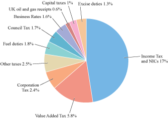
This diagram is a pie chart, divided into ten sections. The data source is the Office for Budget Responsibility, 2012, page 100, Table 4.6.

The largest category of tax is Income Tax and National Insurance Contributions, at 17% of GDP.

Then, moving clockwise the pie chart presents the other categories of tax: Value Added Tax 5.8%; Onshore corporation tax 2.4%; Other taxes 2.5%; Fuel duties 1.8%; Council tax 1.7%; Business rates 1.6%; UK oil and gas receipts 0.6%; Capital taxes 1%; Excise duties 1.3%.

Figure 17 Major UK taxes as percentages of GDP, 2010–11

Taxation is a key component of fiscal policy, alongside government spending decisions, which were considered in the previous section. In a period of economic recession, the government can choose to stimulate aggregate demand by either boosting government spending or cutting taxes. This can be illustrated using the circular flow diagram (Figure 18).

Activity 12

Compare Figure 18 with the circular flow diagram represented in Figure 19.

Figure 18 Government spending and taxation in the circular flow of income

Show description|Hide description

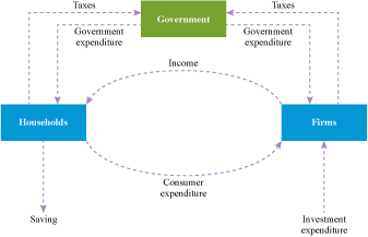
The diagram shows three sectors of the economy, with various money flows shown as moving between them. The money flows are shown as dashed arrows, indicating the direction of flow.

The Household sector is in a blue rectangular box on the left of the diagram; the Firms sector is also in a blue rectangular box is on the right of the diagram; and the Government sector is in a green rectangular box which lies above the other two and in the centre.

From households, consumer expenditure flows to firms and taxes flow to government. There is also a flow of savings from households and this is shown by an arrow pointing out of the circuit of flows – indicating a leakage out of the circular flow.

From firms, income flows to households and taxes flow to government. There is also a flow of investment expenditure to firms. This flows in from outside the circuit of flows – indicating an injection into the circular flow.

From government, government expenditure is shown flowing to both households and to firms.

Figure 18 Government spending and taxation in the circular flow of income

Figure 19 Circular flow of income with investment and saving

Show description|Hide description

Flows of money are shown by dashed lines with directional arrowheads.

A flow labelled ‘Income’ runs from Firms to Households.

A flow labelled ‘Planned Consumption’ runs from Households to Firms.

A dashed line pointing vertically down from Households is labelled ‘Saving’.

A dashed line pointing vertically up to Firms is labelled ‘Planned Investment’.

Figure 19 Circular flow of income with investment and saving

Discussion

You will see that in Figure 18 a new box has been added to show the government sector. As you have seen, government expenditure provides an injection to the circular flow of income, as indicated by the arrows in Figure 18. For example, if the government-run National Health Service hires more doctors, there is a flow of money to the household sector.

Tax receipts are a leakage from the circular flow of income. For example, out of incomes received by households, a part of these are paid in Income Tax, which leaks out of the household sector into the government sector. A reduction in Income Tax would put money into the pockets of households, which could stimulate aggregate demand. Similarly, Corporation Tax is represented here by a flow of money from the firms to the government. A reduction in Corporation Tax could stimulate the expenditure plans of firms.

The leakage of taxes means that there is another important difference between the two models. In the model without government expenditure (Figure 19), planned consumption is the proportion of income left after saving had been deducted; in Figure 18, consumer expenditure is the proportion of income left after saving and also taxes have been deducted.

A tax-modified multiplier

To explore how taxation works as a fiscal policy tool, a modification can be made to the aggregate demand model and multiplier. To keep things simple, we will assume a tax rate for the whole economy, capturing the proportion of income raised from tax. The coefficient t can be defined as the rate of tax – i.e. the proportion of national income levied by tax. Hence the total revenue received by the government from tax (T) is

T = tY

With a national income (Y ) of £1200 billion, for example, and a tax rate of 1/3, the total tax revenue will be £400 billion.

The amount of income available for consumption (often referred to as disposable income) is now equal to income (Y ) minus taxation (tY ):

Y − tY = (1 − t )Y

It therefore follows that the tax-modified consumption function is

C = a + b(1 − t )Y

This tax-modified consumption function, shown in Figure 20, has a shallower slope than the consumption function shown in Figure 14. This new slope is represented by a new (tax-modified) marginal propensity to consume b(1 − t ).

Figure 20 Taxation and aggregate demand

Show description|Hide description

This diagram has Aggregate Demand on the vertical axis and Income on the horizontal axis.

A solid line slopes upwards from the origin at an angle of 44 degrees.

From a point a short way up the vertical axis, a horizontal line is drawn. This is labelled ‘I+G’.

From a point a little higher up the vertical axis, labelled ‘a’, a solid straight line slopes upwards diagonally to the right. This line is labelled ‘Consumption function’ and has the equation C=a+b(1-t)Y. It has quite a shallow slope.

Higher up the vertical axis, from a point labelled ‘a+I+G’, there is another upward sloping line, parallel to the consumption function. This line is labelled ‘Aggregate Demand schedule’ and has the equation AD= a+b(1-t)Y+I+G

Figure 20 Taxation and aggregate demand

We can now consider the effect of modelling tax on the structure of the multiplier, which was shown earlier in this section to take the form 1/(1 − b). It intuitively follows that instead of having a denominator 1 − b, the tax-modified multiplier has a denominator 1 − b(1 − t ). The marginal propensity to consume (b) is no longer the only determinant of the value of the multiplier. We now also need to take account of the leakage of tax, as shown in Figure 20, and the new multiplier is

A tax-cutting fiscal stimulus

It is now possible to explore the impact of cutting the tax rate from t₀ to t₁. Since a higher proportion of income is now available for consumption (a reduced leakage of taxes in the circular flow of income), this provides a boost to aggregate demand. This tax reduction will be modelled in order to illustrate a key fiscal policy arm available to policymakers: the manipulation of taxation in order to stimulate aggregate demand.

In response to a tax cut, the initial reduction in tax payments ΔT is equal to

ΔT = (t₀ − t₁)Y₀

where Y₀ is the level of income before the tax change. The change to tax receipts depends on the difference (t₀ − t₁) between tax rates before and after the change.

Now let the initial level of income (Y₀) be £600 million, and let the initial tax rate (t₀) be 0.1. Suppose that the tax rate falls to t₁ = 0.05 (only 5% rather than 10% of national income is taken in tax). Hence the initial reduction in tax receipts is

ΔT = (0.1 − 0.05) × 600 = 0.05 × 600 = £30 million

The reduction in the tax rate to 5% generates a £30 million cut in total tax receipts. This means a £30 million increase in disposable income.

The ‘windfall’ increase in disposable income will lead to an increase in consumption spending, but this increase will be less than the full £30 million. Assuming that the marginal propensity to consume is 0.8, and remains at this value, households will spend only 80% of their additional income. Instead of stimulating aggregate demand, 20% of the tax windfall leaks into savings accounts in banks and building societies. Hence the stimulus to aggregate demand is

b ΔT = 0.8 × £30 million = £24 million

Households will choose to save £6 million of the £30 million tax windfall, and spend £24 million on additional consumption. So aggregate demand is boosted by £24 million.

In addition, the fall in the tax rate increases the value of the multiplier:

The reduction in the tax rate increases the multiplier from 3.57 to 4.17. The combined effect of these two changes is an increase in income of

4.17 × £24 million = £100 million

The key difference between these two types of fiscal policy is the leakage of part of the tax cut into saving. In the current example, the government spends the full £30 million, whereas households spend only £24 million of the £30 million windfall and save the rest. The exact outcome of the comparison does, of course, depend on the values of b and (t₀ − t₁). The effect of a tax cut will be enhanced if there is a very high marginal propensity to consume, so that most of the windfall is spent, and also if there is a substantial increase in the value of the multiplier owing to a large fall in the percentage tax rate.

Keynes was not very keen on stimulating aggregate demand through tax cuts. As shown by Brown-Collier and Collier (1995), he cautioned that tax cuts do not provide any future benefits to the economy; he also thought that it would be difficult to persuade the public that tax cuts should be reversed once they became established. Further issues relating to these two types of fiscal policy are considered in the analysis that follows.

6.6 Stabilisation policy

You have seen that fiscal policy can be used, in times of economic crisis, to stimulate aggregate demand either by increasing government spending or by reducing taxes. As part of the Roosevelt New Deal, and more recently by President Obama in the USA, these types of fiscal stimulus were used to stabilise the economy in response to problems of severe contraction in national income.

In the golden years of Keynesian economics, however, during the 1950s and 1960s – when the UK Conservative Prime Minister Harold Macmillan pronounced ‘You’ve never had it so good’ – governments did not have to deal with such crises. The news programmes were not reporting people queuing outside banks (as in the 2007 collapse of Northern Rock) or the unemployed queuing outside job centres. Far from there being a problem of unemployment, there was a shortage of labour, which encouraged population movements such as the Windrush migration from the Caribbean to the UK.

For most of this early postwar period, capitalist economies enjoyed continued growth and mild business cycle fluctuations. In such circumstances, there would be repeated periods of boom (high growth) and slowdown (low growth); governments would see their main responsibility as smoothing out the peaks and troughs of the cycle, an approach referred to as ‘fine-tuning’.

This period of sustained growth was attributed in part to the benefits of Keynesian intervention – in sharp contrast to the plethora of disasters that befell the world economy in the 1920s and 1930s. Postwar governments bought into the Keynesian idea that it was their responsibility to manage aggregate demand. In the USA, during the 1960s, the phrase ‘We are all Keynesians now’ (Friedman, 1965) was even used by the right-wing president, Richard Nixon. In the UK, successive Conservative and Labour Chancellors of the Exchequer (Hugh Gaitskell and Rab Butler) were arguably so close to each other that their names were combined in an approach called ‘butskellism’: where the mixed economy, consisting of a viable private sector and a large welfare state, were championed. It was not until the 1970s, when problems of inflation reared their ugly head, that this postwar Keynesian consensus fell apart.

Two main types of fiscal policy were developed during this period. First, governments can use discretionary stabilisers, actively adjusting fiscal policy in response to boom or slowdown in economic activity. If the economy is overheating (growing too fast), for example, the government might decide to increase tax in order to temper aggregate demand – and vice versa under a slowdown. As you saw earlier in this section, the impact of using this type of discretionary stabiliser will tend to be amplified by the multiplier effect. Since for Keynes, in general, the economy is likely to operate at output levels less than full employment, discretionary stabilisers are required to snuff out high unemployment.

Yet if the public sector is sufficiently large, in a butskellite type mixed economy, then its very presence can dampen down the business cycle. If growth slows, for example, and there is an increase in unemployment, then under a welfare state workers will receive unemployment benefit. So although they are not earning the wages that they earned under employment, unemployed workers are still able to consume, albeit at a lower level. Such a transfer payment can be thought of as a negative tax, affecting consumer expenditure in a similar way to a tax cut.

This second type of fiscal policy is referred to as an automatic stabiliser – a fiscal response to a slowdown in economic activity that happens without any active decisions on the part of the government. Governments, of course, have to choose to keep the system in place to facilitate this automatic spending, but they do not have to actively direct the spending from day to day.

At the same time as government transfer payments will automatically increase during a slowdown, tax revenue will fall. At lower levels of income, tax receipts such as those out of income (Income Tax) and profits (Corporation Tax) will fall. The welfare and tax systems in the economy create their own adjustments in aggregate demand, making the slowdown less pronounced than it would have been without the state sector. Similarly, in an upturn, as incomes increase so does the proportion of income directed to tax.

In recent years, policymakers have found these stabilisers to be very attractive, since they can smooth out both peaks and troughs of the business cycle. Tax-based automatic stabilisers provide a symmetric approach to fiscal policy, with attention paid to both sides of the business cycle. In the early 2000s, this was the official position of the European Central Bank (ECB): ‘Automatic stabilisers are the appropriate way to stabilise output, as they have foreseeable, timely and symmetrical effects […] there is normally no need to engage in additional discretionary fiscal policy-making for stabilisation purposes’ (ECB, 2002, pp. 41, 46, quoted by Lodewijks, 2009, p. 3).

This contrasts sharply with the Keynesian consensus of the 1960s, when it was thought that automatic stabilisers were insufficient to manage the business cycle. US President John F. Kennedy argued in 1962 for a ‘shelf of public works’ that could be introduced if unemployment rose – together with increases in the period for which unemployment benefits would be paid (Lodewijks, 2009, p. 4). The problem, for the USA, is that state spending has tended to constitute a smaller part of national income than in European countries such as the UK, so automatic stabilisers do not have as much impact.

Despite its weaker automatic stabilisers, the USA enjoyed a stronger recovery than the UK in the period immediately following the economic crisis of 2008. Adam Posen, a member of the Bank of England’s Monetary Policy Committee, has explained this recovery as being in part due to differences in the discretionary fiscal policy:

While Obama introduced a fiscal stimulus, the Conservative/Liberal Democrat Coalition in the UK implemented a fiscal contraction. Posen pays particular attention to the increase in VAT announced by Chancellor of the Exchequer George Osborne in his emergency Budget of 22 June 2010, from 17.5% to 20%. Posen argues that this VAT rise helps to explain the fall in private consumption since the peak of the business cycle, compared to the USA, as shown in Figure 21 by the divergence of the two lines after Quarter 10. The argument is that the increase in VAT, and its anticipation by consumers, led to lower consumer spending, which spilled over to fewer jobs and lower income throughout the economy.

(Source: Posen, 2012)

Figure 21 Percentage growth rates of private consumption in the UK and the USA, following the economic crisis of 2008

Show description|Hide description

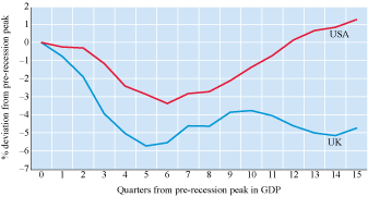
This diagram is a time series line chart. The data source is Posen, 2012.

The vertical axis is labelled ‘Percentage deviation from pre-recession peak’ and is marked from minus 7 to plus 2, at intervals of 1. The horizontal axis is labelled ‘Quarters from pre-recession peak in GDP’ and is marked from zero to 15 in intervals of 1.

There are two lines on the chart, one for the USA and one for the UK.

Both lines start at zero on the vertical axis. The line for the USA is above the line for the UK at all points thereafter.

The USA line declines steadily to a low point of just below minus 3%, in the sixth quarter from the pre recession peak in GDP. It then rises steadily to reach plus 1% in quarter 15.

The UK line declines to almost minus 6% in quarter 5, rises slightly to minus 4% in quarter 10 and then declines again to minus 5% at the end of the period.

Figure 21 Percentage growth rates of private consumption in the UK and the USA, following the economic crisis of 2008

6.7 Government debt and crowding out

You have discovered that governments can boost aggregate demand either by increasing government spending or through cutting taxes. There is, however, an elephant in the room, which you must have noticed, and this section has so far studiously ignored (just to keep things simple): how can a fiscal stimulus be paid for? Surely if the government spends more to get the country out of a crisis, it runs the risk of squeezing the private sector, or even worse, bankrupting itself. These two issues are considered first by looking at government debt, before turning to a consideration of how the private sector can be squeezed by government spending.

The debt problem

This common sense mantra has been espoused by those on the right of the political spectrum in response to the economic crisis of 2008, such as the Tea Party movement in the USA. The alternative political position is captured in the T-shirt below, worn by supporters of the anti-cuts movement.

Figure 22

Show description|Hide description

Photo of T-shirt. Printed on front the words 'The cuts won't work, they'll just make it worse'.

Figure 22

Rather than spending in a recession, the government orthodoxy (traditionally referred to as the ‘Treasury view’ or ‘sound finance’) has been to balance its budget by cutting expenditure. This ‘sound finance’ view, traditionally associated with the nineteenth-century Liberal Prime Minister William Gladstone, is not limited to recessions. It more generally states that the government budget should be balanced at all times (or in slight surplus so as to pay down past debt).

The balanced budget approach has been the cornerstone of the Conservative/Liberal Democrat coalition government since coming to power in 2010. With a target to balance the budget by 2016, it introduced a programme of severe cuts in government spending. In his 2010 emergency Budget, George Osborne proclaimed:

The coalition government also argued that they inherited the largest level of debt incurred by a British government during peacetime. As shown in the box opposite, when the last Conservative/Liberal coalition was in power, led by Lloyd George (before he became a Keynesian), a similar austerity programme, known as the Geddes Axe, was implemented.

The Geddes Axe: a brief explanation

Figure 23 An unemployed man and his family on the streets of Brighton in 1921 (Photo: Associated Newspapers/Daily Mail/Rex Features)

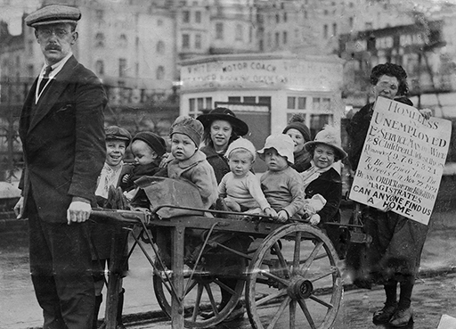
After the First World War, Britain was gripped by enormous debts and a growing sense of panic that the Government was hugely wasteful.

The national debt had risen dramatically from £677 million, about a quarter of the GDP, in 1910. By 1920 it was £7.81 billion, larger even than the country’s GDP. A vast civil service, that had come together to administer the war effort, was still operating at full capacity, while spending on education had increased substantially. Many of the middle classes complained how their tax bills had shot up.

The Government was under pressure to do something. The Times newspaper noted in 1922: ‘There are signs of an astonished realisation of the alarming bill for civil pensions that in a few years will be a millstone on the taxpayer’s neck.’

The Anti-Waste League, formed by Lord Rothermere, had put up candidates and won three by-elections during 1921.

David Lloyd George, the prime minister, acted by appointing a businessman Sir Eric Geddes to head the new Committee on National Expenditure, which was soon dubbed ‘The Great Axe’. It highlighted waste in all areas of public spending, including details such as there being a ratio of one cleaner for every vehicle in the Army. Between 1921 and 1922 it recommended economies totalling £87 million, about 10 per cent of the country’s entire GDP.

Though the cabinet only agreed to £52 million of cuts, these were enormous for the time and in the end, total cuts were larger than either of these figures. He was hailed a ‘superman’ by one leading businessman, but the axe hit some people very hard and led to a large reduction in social benefits, particularly secondary education.

The biggest cuts were in the Army and Navy. The defence budget was cut by 42 per cent in the space of one year. But other workers were hit too.

Civil Service numbers were cut by 35 per cent – mostly female staff hired during the war.

At the close of 1921, wage cuts averaging 8 shillings a week had been imposed on 6 million workers. This equates to a £58 fall in today’s money and led to growing anger against the government.

The cuts were driven by a Treasury desperate to keep a control of its debts, but they partly caused Britain’s woes in the 1920s – a period of far greater economic trouble for the country than it ever experienced during the 1930s. The General Strike in 1926 can, in part, be explained by the mounting resentment caused by the cuts, though some economists argue it helped Britain exit the vicious recession of 1919 to 1921 quicker than it might otherwise have done.

The Geddes Act, introduced by one of the great Liberal administrations, ironically gave impetus to a burgeoning Labour Party. The number of seats it held rose from 59 in 1918 to 142 in 1922, reflecting a new coalition across class lines. It went on to form its first administration in 1924.

(Source: Wallop, 2010)

It was in the aftermath of the Geddes cuts in the 1920s that Lloyd George and Keynes formulated their arguments as to why governments could spend their way out of recession. Keynes once said ‘When the facts change I change my mind. What do you do, sir?’ – a mantra that would equally apply to Lloyd George during this period. Keynes also argued that a government spending programme could be easily paid for, without threatening government finances.

Thus far this section has made reference to both a budget deficit and government debt. It is important to be clear about how these differ.

Government debt, also called the national debt, is the total amount of money owed by the government to all those from whom it has borrowed. It is a stock, that is, an accumulated amount, not an amount measured per period of time.

The primary budget deficit is the excess of government expenditure over tax receipts in a given time period, usually one year – so it is a flow. In any year when there is a deficit, the national debt will increase. If there is a budget surplus (tax receipts exceed expenditure), then the government may decide to use part of it to reduce its outstanding debt. If tax receipts exactly match government spending, then this is referred to as a balanced budget.

Balancing the budget

The policy of balancing the budget can be looked at from a Keynesian perspective. Suppose that the government increases its spending by £30 million and balances this increase by raising £30 million in taxation. To earn this additional revenue from tax, the tax rate is increased from 5% to 10%. The economy starts at an income level of £600 million. The overall effect can be analysed in three steps.

Keynes and government debt

Keynes recognised the need, in times of crisis, for government borrowing to finance a sizeable expansion of government spending. The government traditionally borrows by issuing loans (referred to as government bonds or gilts) that it promises to pay back at a future date. In the meantime, interest is also paid to holders of these bonds.

Let i be the rate of interest paid on government bonds. If a bond worth £100 is issued by the government and bought by a private individual or bank, then after one year the government will pay out a percentage rate of interest. Say the rate of interest is 6%; this means that the government pays out £6 after one year. The total value of bonds (debt) issued by the government can be denoted by the term D. Thus the total interest payment made by the government is iD.

If the total amount of debt owed by the government is £300 million, for example, then the debt repayments in a particular year would be

total interest payments = 6% × £300 million = £18 million

It follows that the total government deficit is the primary deficit (government spending minus taxation) plus these debt interest payments

total deficit = government spending − taxation + total debt interest payments

This is the total government deficit that economists and policymakers usually worry about. In a more compact notation, the total deficit is

G − T + iD

In the case of Greece, during the European financial crisis that started in 2010, the main problem has been trying to service the interest payments on its debt. This problem has been compounded by the lack of confidence in Greek bonds in the world financial markets.

The ‘sound finance’ advice given by policymakers, in the European Commission and beyond, has been for Greece to cut government spending and increase taxes in order to meet its debt interest payments. From the perspective of Keynes, however, the problem with this austerity approach is that the reduction in government spending will, via the multiplier, reduce national income and the ability of the economy to generate tax revenue. In the face of this type of crisis, Keynes would have called for the government to boost income using government infrastructure spending.

Take, for example, the Liberal spending programme of £300 million in 1929, referred to earlier in the section. Keynes assumed that the government would have to take out a loan (i.e. issue bonds). Assuming that it had to pay interest of 6% on this loan, then in the first year of the spending programme government would have to meet debt interest payments of £18 million. The key question is how these debt interest payments can be covered. Using the multiplier, one can specify what happens to income and taxation receipts.

The tax-modified multiplier relationship takes the form

The multiplier captures the impact of a change in government spending (ΔG) on national income (ΔY).

For the fiscal stimulus of ΔG = £300m, the change in income would be

ΔY = 1.5 × 300 = £450m

This means, taking into account the leakage of income into taxation, that a multiplier of 1.5 leads to a £450m increase in income, in response to the £300m increase in government spending.

Now what is the impact, in this example, on receipts from taxation? In the aggregate demand model there are additional receipts from taxation (ΔT ) since the income out of which taxation is paid has increased

ΔT = t ΔY = (1/3) × 450 = £150 million

The amount of tax paid out by the national economy increases by £150 million, since there is more income available out of which to pay taxes. The government has put an additional £150 million into its coffers. For Keynes, this shows that his public expenditure increase of £300 million is affordable. With tax receipts increasing by £150 million, the £18 million of debt interest payments on the government’s infrastructure loan can easily be covered.

But what about the deficit? In this example, the deficit increases by £150 million since only half of the £300 million outlay is recouped in tax receipts. There has been no increase in the tax rate to balance the budget, as before. However, Keynes distinguished between current and capital expenditures. Current expenditures are used up in the short run, when capital stock, among other things, is fixed. In contrast, capital expenditure is expenditure made on items that are available for future use, in the long run: a period of time in which the capital stock can change. For Keynes, investment in infrastructure is not included as part of current expenditure or of the current fiscal deficit. Investment, for example in transport, would provide an increase in the assets of the country, helping the productivity of private firms, enabling them to transport their goods to customers (as would investment in education).

So for Keynes investment can be earmarked for a separate wealth-creating part of the national accounts: ‘It is not the miser who gets rich; but he who lays out his money in fruitful investment’ (Keynes, 1972, p. 123). On this basis, the investment in infrastructure could be classified as improving the health of the public sector accounts. If the accounts were in surplus, the new tax receipts would add to that surplus; if the accounts were in deficit, the new tax receipts would be used to pay off the country’s debt. Out of the £150 million tax receipts, £18 million would be used to cover debt interest payments, but a clean £132 million would be added to government coffers. For Keynes, you can spend your way out of debt, contrary to the quotation from Daniel Hannan earlier in this section (see 'The debt problem').

When is debt high?

In modern economics, however, funding capital expenditure is usually included in the calculation of government debt and deficits. In response to this constraint in the UK, governments have introduced schemes such as the Public Finance Initiative (PFI), in order to classify funding public infrastructure spending as private debt.

But even if this orthodox classification of capital spending is accepted, it can still be argued that the Treasury view, under which government spending is cut in order to balance the budgets, is misguided in times of recession. Rather than viewing this approach as ‘sound finance’, it can alternatively be labelled ‘debt alarmism’ or ‘fiscal scare tactics’. In this vein, Neild (2012) has compared gross levels of debt in the UK since 1816, as shown in Table 2.

Neild (2012) makes three main points. First, the gross debt for 2010 of £1 071 000 million – just over one trillion pounds – is a large amount of money, and can easily make its way into the headlines, but it is not so high in historical terms. To show why, Neild examines what economists call the ‘debt to GDP ratio’ (ratio of total debt outstanding to GDP). In 1816, just after the Napoleonic Wars, this amounted to 260%; after the First World War, in 1919, it was 127%; after the Second World War it amounted to 225%. So the 75% of GDP in 2010 does not look so alarming in this historical context. Keynes argued that British governments are far too unwilling to spend during times of peace. They are often willing to wage a war on the French or Germans – but when it comes to attacking unemployment, governments are unusually peace-loving in their expenditure plans.

Second, there has not been one occasion during this period, argues Neild, when the British government has failed to borrow what it requires to meet spending requirements. Not when Napoleon was hauling cannon across Europe; not when the Kaiser transported a million men to the French border on his newly built railways; not even under Hitler’s Blitzkrieg. No matter how much money Britain needed to borrow to face these threats, it did not fail to raise debt. It is somewhat alarmist, Neild and others argue, to pronounce that the British government is in danger of going bankrupt. For some this is a fiscal scare tactic used to justify an ideological prejudice against the public sector.

Finally, Table 2 is used by Neild to show the dangers of cutting government expenditure in an attempt to reduce debt. In 1923, after the Geddes Axe, the ratio of debt to GDP went up to 176% from 127% in 1919, as GDP fell from £5.83 thousand million 1919 to £4.39 thousand million in 1923. Unemployment, as shown in the table, increased from 3% to 12% over the period 1919–23. Similarly, a series of cuts by the Ramsay MacDonald government in the early 1930s, which Keynes railed against, led to a reduction in GDP from £4.73 thousand million in 1929 to £4.26 thousand million in 1933. The debt to GDP ratio increased from 158% in 1929 to 179% in 1933, with unemployment rising to 20%. For Neild, as also argued by Keynes, debt problems (as expressed in the debt to GDP ratio) are caused in peacetime by low GDP – not by wasteful spending by governments.

The Keynesian argument is that cuts in government spending can lead to an increase in the fiscal deficit; the best way to reduce deficits is by increasing output, and this can at times require injections of aggregate demand from discretionary fiscal policy. But this has not been the consensus among policymakers. The European Union, for example, has sought to put severe constraints on fiscal policy. Under the Stability and Growth Pact, set up in 1996, European countries were set a target for government deficits of 3% of GDP, and could be fined if this was transgressed. So when a recession comes along, even the automatic stabilisers must be taken off the policy bike if the 3% target is breached.

This inflexibility led to a relaxing of the 3% target in 2005, in order to allow for business cycle fluctuations. As shown in Table 3, in the economic crisis that swept across Europe, by 2010 even Germany, one of the most fiscally conservative of the European Union members, was unable to meet the 3% target. The entry −4.3 shows that in 2010 Germany had a fiscal deficit (indicated by this being a negative number) at 4.3% of GDP; in 2007 Germany had a surplus of 0.2% of GDP. In 2007, before the recession took hold, all the countries shown in Table 3 (apart from Greece) were either in surplus or had deficits that were within the 3% target. It was the combination of collapsing GDP and the use (automatic and discretionary) of fiscal stabilisers that led to the breaking of the target. The key question for macroeconomists is whether a more austere fiscal policy at the time would have worsened or reduced the deficit.

Crowding out

A further criticism levelled at the Keynesian fiscal policy is the risk of crowding out. This is the idea that government spending may squeeze out consumption and investment by the private sector, so that the growth in aggregate demand from an increase in G is at least partially offset by a fall in C and/or I.

A key proponent of the idea that government spending may crowd out consumption is the economist Roger Farmer. His arguments start with a way of looking at the consumption function that is different from the familiar Keynesian one in which consumption is determined largely by income (Farmer and Plotnikov, 2012). The alternative is based on an approach developed by Milton Friedman called the permanent income hypothesis (Friedman, 1957, pp. 21–2). In Friedman’s view, consumption is closely linked to wealth rather than income. People take a long view and set a normal level of consumption according to their wealth. This means that people may borrow now to support a high standard of living if they expect their earnings to rise in future (because of, say, the anticipated rewards from their education, training and experience), or they may limit their consumption now in order to save enough for a comfortable lifestyle later when income is expected to drop (typically after retiring).

The gist of Farmer’s argument is that if the government announces an increase in government spending, G, then households will expect this to mean a rise in taxes, T, later (whether to bring the government’s budget back into balance or to pay off government debt used to fund the increase in G). Given their long view, households will offset the gain to themselves from G today against the future loss in T – and so increase their savings to cover the expected future tax bill rather than increasing consumption, thus partially or completely offsetting the rise in G.

Barro (1981) also points out that many types of government spending can be seen as close substitutes for private-consumption goods – for example, a public health service (like the NHS in the UK) is a substitute for private medical care, unemployment benefits are a substitute for private insurance, publicly funded schools and universities are substitutes for private education, and so on. If the government increases spending on these types of items, then consumers will cut back on the amount that they spend privately on similar items.

Keynes offered an explanation of how government borrowing to fund a rise in G could crowd out private investment:

If the government issues too many bonds, then it may have to increase the rate of interest in order to find buyers. This is what happened to Greece and Italy, from around 2010. The high interest rate in these countries would have had an adverse impact on the level of private investment; hence some would argue that government overspending crowded out the private sector.

However, for some countries, such as the UK and the USA, this argument may not apply. For some time after the 2008 crisis, interest rates languished at low levels, despite high deficits. Economies are often more complicated. A major factor determining the effectiveness of fiscal policy is the confidence that international markets have in government-issued debt and animal spirits. As Keynes puts it:

6.8 Summary

In Section 6, a lot of time has been spent on placing Keynes’s aggregate demand approach in its historical context: from the austerity of the 1920s and 1930s, to the golden age of Keynesian economics in the 1950s and 1960s, to the obsession with deficits since the 1990s. This is for two main reasons. First, it is important to have a feel for where ideas come from, and why economists and policymakers have considered them to be important – to give you a foundation in the discipline of macroeconomics and its place in political economy. Unemployment was the key prewar illness, and Keynes is the economist said to have developed the required medicine, which became the basis for postwar policy. This is the backdrop to modern macroeconomics as we know it.

Second, the spectre of unemployment has come back with a vengeance since the economic crisis of 2008, and Keynes also has made something of a comeback. His ideas are suddenly relevant again. The debates that took place in Keynes’s time – about whether fiscal policy can work, the fiscal stabilisers available to the government, whether governments can afford to stimulate aggregate demand, and whether they should instead cut spending in order to reduce the deficit – are all highly relevant to recent debates throughout the world.

7 Zooming in on firms

So far, we have concentrated on the study of macroeconomics, but have not focused on the economics of individual firms or markets. To understand microeconomic theory, we study the activities of firms, their production processes and the markets where goods and services are traded. The idea of firms and production should be familiar to you, for instance, when we discussed how changes in the level of investment by firms influences aggregate demand and overall GDP. Section 7 will explore the activities of firms in more detail. We will begin to look at activities such as how production processes can be modelled in economics, and how the prices of specific goods and services – the market price – depend on how much firms are willing to supply, but also the quantity which consumers are willing and able to buy.

The section examines how firms can grow by increasing output and reducing cost. It looks at how production can be organised efficiently, and also shows that in any market there will be winners and losers. The economic theory in the section is closely linked to examples of real firms and markets that can be used to demonstrate how you can apply microeconomic theory to everyday news and events. It will help you to understand why the price of fresh food rises when supply is scarce, and why some firms make large profits while others struggle to survive.

7.1 Facing the competition

Activity 16

Examine the three figures shown below. Pause for a moment and consider what story they tell us about how these two economies are performing.

How do you think the macroeconomics relate to the performance of firms in these two countries?

(Source: Eurostat, 2013a)

Figure 24 Real GDP performance as an index (base year = 2000)

Show description|Hide description

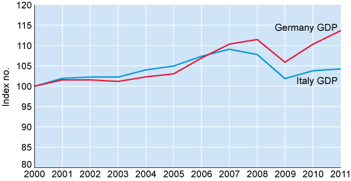
This diagram is a time series line chart.

It has ‘Index number’ on the vertical axis, running from 80 up to 120 in intervals of 5.

The horizontal axis shows the years, running from 2000 on the left to 2011 on the right.

There are two lines shown on the diagram, one labelled ‘Germany GDP’ which is in red and the other labelled ‘Italy GDP’ which is in blue.

Both lines start at 100 on the vertical axis. They both rise steadily, staying close together, to reach around 110 in 2007. From 2007 the lines diverge. The Germany GDP line continues to rise a little to 2008 and then falls to just over 105 by 2009, before rising quite sharply to reach 115 by 2011.

In contrast, the Italy GDP line falls to about 102 in 2009 and then rises but only very shallowly to just reach 105 by 2011.

The data source is Eurostat 2013a.

Figure 24 Real GDP performance as an index (base year = 2000)

(Source: Eurostat, 2013a)

Figure 25 Export component of GDP as an index (base year = 2000)

Show description|Hide description

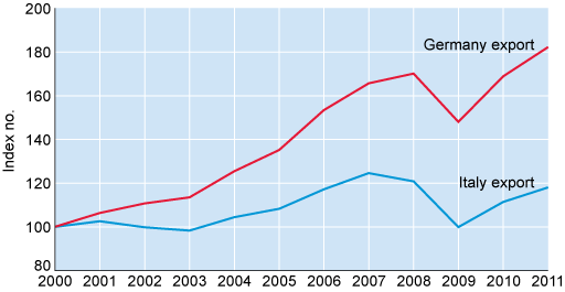
This diagram is a time series line chart.

It has ‘Index number’ on the vertical axis, running from 80 up to 200 in intervals of 20.

The horizontal axis shows the years, running from 2000 on the left to 2011 on the right.

There are two lines shown on the diagram, one labelled ‘Germany export’ which is in red and the other labelled ‘Italy export’ which is in blue.

Both lines start at 100 on the vertical axis but then diverge immediately. The Germany export line rises steadily to reach 170 by 2008. The line then falls steeply to about 150 in 2009 before rising steeply to reach just over 180 by 2011.

The Italy export line is pretty flat to 2003, it then rises to reach just over 120 by 2007. The line shows a sharp fall back down to 100 in 2009 before rising to reach 120 by 2011.

The data source is Eurostat 2013a

Figure 25 Export component of GDP as an index (base year = 2000)

(Source: Eurostat, 2013b)

Figure 26 Unemployment performance

Show description|Hide description

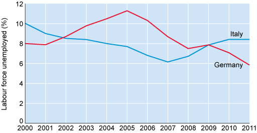
This diagram is a time series line chart.

It has ‘Labour force unemployed (percent)’ on the vertical axis, running from 0 up to 12 in intervals of 2.

The horizontal axis shows the years, running from 2000 on the left to 2011 on the right.

There are two lines shown on the diagram, one labelled ‘Germany’ which is in red and the other labelled ‘Italy’ which is in blue.

The Germany line starts at 8% in 2000, then rises steadily to around 11% in 2005 before falling to just under 8% in 2008. The line then rises slightly to 2009 before falling quite steeply to 6% in 2011.

The Italy line starts higher up, at 10% in 2000. It then falls steadily to below the Germany line, to reach 6% in 2007. From 2007, the line rises steadily to reach just over 8% by 2011. As it rises, it crosses the Germany line in 2009.

The data source is Eurostat 2013a.

Figure 26 Unemployment performance

Answer

The three figures above give a brief overview of the recent performance of the Italian and German economies. They suggest a contrasting economic performance. From 2007 the performance of Italy’s GDP has fallen behind Germany’s, as shown in Figure 24, particularly in the period following the economic crisis. Over the last decade, Germany has continued to improve its export performance, whilst Italy’s export levels have struggled to increase beyond the level in 2000. Interestingly, the unemployment rate in Germany has fallen since 2005, having started at a much higher rate than in Italy. Germany’s unemployment has continued to fall, even in the period following the economic crisis. In contrast, unemployment in Italy has remained between 6–8 per cent, and increased starting from 2008.

The difference in performance at a macro level may suggest some insight into the aggregate performance of firms in each country; it may suggest that German firms have some advantages over their Italian counterparts. For instance, investment in human capital in a country should help to increase the productivity of firms and make them more competitive internationally. So we might expect German firms, on average, to perform better than their Italian peers. However, even if there are differences in the macro performance of two countries, when we look at the micro level, we may be able to detect common characteristics of firm behaviour that can be related to higher performance, whether firms are based in Italy or Germany.

Firms in Italy and Germany

Activity 17

Watch the following video, Facing the competition, which examines how firms in Italy and Germany are facing up to strong international competition. Then answer the questions below.

Download this video clip.Video player: Facing the competition

Show transcript|Hide transcript

Transcript: Facing the competition

NARRATOR

The rise of low wage manufacturing has fundamentally changed the nature of international competition. Firms in western economies with higher wages and costs have struggled to remain competitive. This film explores how firms in two of Europe's largest economies - Italy and Germany - are facing up to competition from low cost international producers. Should they force down their own costs, or are there other ways they can compete?

Historically, the two countries have taken very different routes towards improving industrial competitiveness. The German success story in exporting manufactured goods is well documented, but less well known is Italy's track record.

SANDRO TRENTO

Italy is among the top exporter in the world. We are the second largest manufacturing country in Europe. After Germany, there is Italy as the largest manufacturing sector in Europe.

NARRATOR

Before the introduction of the euro in 1999, the Italians relied on manipulating their currency.

SANDRO TRENTO

Up to the nineties, the Italian economy could gain competitiveness through the devaluation of the Italian lira, the currency. That gave competitiveness gain to the Italian industry.

NARRATOR

After Italy joined the euro, devaluation was no longer an option, and structural economic changes were vital to improve competitiveness and economic growth.

SANDRO TRENTO

The real problem is growth. We have a very bad performance in terms of GDP growth. Most of the problem are micro, labour market, firm size, education. If the justice sector is very inefficient, if the state sector is very inefficient, if transportation are not very efficient, the easiness or the difficulty to make business, enforcing contracts, getting credit, they are very difficult to solve in Italy compared to other advanced economies. Most of the problem, the urgent problem, are micro economic today.

LUIGI ORSENIGO

Productivity has been stagnating for over 20 years now, whereas in other countries, it has been growing at higher rates. There has been very little investment, especially in training, R&D, not necessarily stand up, high sky R&D, but day-to-day operations. I remember 28 years ago, when some friend of mine and I were complaining, saying, listen, we're spending too little in this kind of investments. We are going to suffer. Here we are.

MARIANA MAZZUCATO

Italy has not actually made the kind of investments that countries like Germany have been making in human capital, in research and development, in different variables that increase productivity. Fiat has not been investing in new engines at the same level that Volkswagen has.

NARRATOR

Low productivity has meant Italian companies have struggled with competition from countries with lower labour costs. In textiles, Italy is a significant exporter but, over the last 20 years, cheap clothes and fabrics from Asia have had a big impact on sales.

FERNANDO ALBERTI

In the nineties and the first years in 2000, this was the most horrific time: 2005 is actually the turning point, where most of the companies which were not prepared in order to compete very fiercely and strongly towards survival, they started to fail.

NARRATOR

Italian companies across all sectors tend to be smaller than their competitors, making them more vulnerable: 95 per cent have fewer than ten workers.

FERNANDO ALBERTI

If we take the typical size of furniture company in Italy, it's about six employees. If we take the average size of German firms in furniture, it's sixty employees, so it's one to ten in comparison. And this, I think, is important in many respects, especially when it comes to face the global competition.

NARRATOR

Small firm size makes it difficult to invest in new technology and exploit economies of scale. The companies that have proved most resilient have controlled costs and been the most innovative. Biella - an historic textile district in northern Italy. Giovanni Germanetti is a family owner of a medium-sized woollen and cashmere business that has survived.

GIOVANNI GERMANETTI

In Biella, many companies have closed down in the past years. Most of the competition came from Eastern Europe and China because in those countries, the labour force is much, much cheaper than in Italy. The people who are doing higher stuff has stayed in the market. The people who are doing very lower stuff, they have been taken over from China.

NARRATOR

And in Prata, a famous Tuscan textile district, the changes were even more dramatic. When Italian businesses went bust, Chinese entrepreneurs took over the factory space with Chinese workers on lower wages than the surviving Italian companies. The Chinese were keen to exploit the 'Made in Italy' label. Initially, they supplied Italian businesses with cheaper fabrics and clothes but, once established, they began to directly compete with the Italians at the low end of the market.

NARRATOR

Although Italian clothing firms at the low end have been wiped out, there's still a strong global market for Italian high end textiles. But there's also a heightened awareness that even these businesses cannot afford to be complacent.

NARRATOR

In Germany, like Italy, family firms form the backbone of the economy. The so-called mittelstand of small and medium sized companies employ over 60 per cent of the labour force. But, unlike Italy, there's a strong history of high investment.

GERNOT NERB

We have quite a few medium sized companies which are very successful. Often, they are world champion in a specific niche. In Germany, the companies normally stick to their main product line or improve it, of course, and leave the money there, and I think this reinvestment by the owners is helping them to be successful.

NARRATOR

One of Germany's most successful companies is Miele. Set up in 1899 to make high quality butter churns, it's evolved into a premium white goods manufacturer, selling high end washing machines and household appliances around the world.

MARKUS MIELE

We have a higher quality. We test the appliances to last 20 years, and this means we have to charge a higher price for that. We have just one brand, and this is different to most of the competitors in the white goods industry. They have a lot of brands.

MARKUS MIELE

We charge a higher price, but we have the quality and we have the features inside. And this strategy has served us well for more than 100 years.

NARRATOR

Like many mittelstand companies, Miele invest in high levels of R and D, to keep up quality levels, but also to create new and improved products.

MARKUS MIELE

Innovations are very, very important in the white goods industries, like our honeycomb drum, for example, in the washer. So you have to add something in order that the consumer says, wow, this is really a great machine. So we have to constantly innovate, and we spend between five to seven per cent of the whole turnover on research and development, which is quite a lot. So you have to invest.

Sometimes, features or products do better than others. We also have products which are not successful, of course. We also stop products where we said we don't make much money on them.

NARRATOR

Despite charging high prices to cover their investments, Miele are conscious about costs and maximising profits.

MARKUS MIELE

We have to really look into every detail and see how can we optimise costs. Sometimes, we have to automate. Sometimes, we have to find different solutions, but in the end, you have to also look at profitability. So what's the most profitable point for your company in the market? Economies of scale are important, but sometimes they stop for the premium positioning, for example. And then you go into the mass market, which others can do much better than we do, so you have to observe what is the right point for your company, concerning sales quantities, and so on.

NARRATOR

The German economy is currently flourishing but, ten years ago, in the early 2000s, growth was stagnant with high unemployment. This led the Schroder government to introduce labour market reforms, including cuts to unemployment benefit.

GERNOT NERB

This put pressure on employees to take up jobs which are less well paid than they used to be. Also, the temporary work became a very important element, and this gave lots of flexibility to companies like - if you take companies like BMW or others - they employ almost one-third of their staff with the help of such agencies.

NARRATOR

But just how important were the Schroder reforms for improving German competitiveness?

MARIANA MAZZUCATO

Alone that would have never, in and of itself, allowed Germany to produce the kind of goods that the world wants to buy. I think it's really in combination with the investments that Germany was making in R and D, in human capital, and its varied institutional structure that those Schroder reforms had an effect. Instead, what we're hearing today is that, if the weaker eurozone countries want to grow and to be like Germany, then they should hold down wages, as if that was the only source of its success. That is a very ideological interpretation of the German miracle.

NARRATOR

Back in Italy, many of the textile companies that have survived have adopted an approach with similarities to that of the German mittelstand, by targeting the high end of the market.

NARRATOR

Lenzi Egisto used to specialise in shoes but, after being undercut by the Chinese in the 1990s, they shifted to collaborating with American company DuPont on new textile innovations.

ROBERTO FENZI

DuPont was producing very nice fibres, very nice yarns, and they had a gap between the yarn and the end user. And we were the link between those two points, so we become a sort of operating lab, receiving the special fibre, making the fabric. Thanks to this operation, we went in touch with some of the major brand names, offering very high tech materials, but with a very fashion look.

NARRATOR

Over the last ten years, Lenzi have developed a series of innovative textile based products, including bulletproof clothing, protective footwear, and specialised fabrics for the health and fashion sectors. More and more companies are also opting for vertical integration, where all stages of production are kept in-house, as much as possible, to ensure consistency and top quality.

ROBERTA RABELLOTTI

We've a very important process of selection of companies, the good firms have survived, and probably the bad or so-and-so firms have now disappeared. So, from this point of view, this could even be a good sign for the future.

NARRATOR

Another growing trend in both German and Italian manufacturing is to take a much more global perspective on production and on sales.

MARKUS MIELE

In 1994, we still had a share of 50 per cent in Germany and 50 per cent abroad. Now, last year, it was 30 per cent Germany and 70 per cent abroad, although we were growing in Germany. This means, if you think about development for example, that people have to think much more about the needs of the consumers outside Germany. With 47 countries where we're selling, we have to make sure the products we produce have the right features for the right consumers in those countries. So it's not only Far East, it's not only Italy, it's not Germany any more. It's a worldwide competition.

NARRATOR

Part of meeting that competition has been to offshore some of the labour intensive aspects of the production process, to save costs. But this can threaten the quality control of companies that are used to high levels of vertical integration.

MARKUS MIELE

We have factories, also abroad, where we manufacture parts and sometimes also whole appliances for Miele, but always the same quality level. So the most difficult decision is to find the right persons to run that factory because they have to understand how we think about quality, what we want the product to look like, and if they can really get our spirit. Once they got it, then it's not a problem, and then you can run a factory in almost any country.

NARRATOR

And even in Italian textiles, where the 'Made in Italy' label is crucial, there's a growing trend to offshore at least the early stages of production.

GIOVANNI GERMANETTI

We have invested 15 years ago in Poland, and we have a spinning mill over there where we produce part of our yarn that is used in our weaving facility. When we started 15 years ago, it wasn't easy, and they didn't have that know-how that we had in Biella. But things were going so expensive for the labour force in Italy that we were obliged to move to Poland. And so now, after a long time of training our employees, we can say that we achieve the same level of quality as we do in Italy. But if the production, the weaving, and the finishing is done in Italy, it's made in Italy.

NARRATOR

And some Italian textile companies have taken a step further by developing international partnerships.

ROBERTA RABELLOTTI

This is an important strategy for the competitiveness of Italian firms. Probably it's less widespread than one can imagine, and this is due to the small size of Italian companies, but the successful companies, companies which have been able to scale up and to outsource. And this is, of course, very important in terms of reducing cost.

ROBERTO FENZI

We have found a very profitable cooperation with the Chinese. And so Chinese are not always an enemy, but they can be an opportunity because, for Lenzi, China is a good customer. It's a good partner. They want a local service. They want a logistic to buy directly from China. Doesn't matter if it is made in Italy or somewhere else. The problem for them is to buy China on China.

NARRATOR

But although many companies have made those international partnerships work, they're not always successful.

HAGEN REIMER

The skills are not something you can just train people on for a year or a few month and then expect them to work like workers who have been doing this for years or even for generations, in Germany. For example, there's a big manufacturer of bearings for industry needs and for automotive, and he pushed production a few years ago to Romania. And he send German people to train the workers there on the job, and it just didn't work out. They lost millions of euros, and then, finally, they decided to get their production back here because it just didn't work the way it was supposed to.

NARRATOR

Another danger is that international partnerships seem to speed up the process of catch-up with Italy and Germany, even at the high end of production.

GERNOT NERB

We did a study some years ago to what extent China could be a competitor for German high-tech industry. Well, at that stage, we thought it will take at least 10, 15 years before they catch up but, nowadays, we have to face the problem that, in some areas, the Chinese are catching up faster than expected. This makes it necessary that we push ahead in the field of innovation in order not to lose the technological leadership.

NARRATOR

This film has shown that, despite their very different economic contexts, there are some striking similarities in the way the strongest Italian and German firms compete on the global market.

FERNANDO ALBERTI

We notice that those companies that are much more performing compared to others, they have the same kind of patterns. So first of all, they [are] innovating in the products, these companies are companies that continuously introduce new kind of products. The second thing is process innovation, so they continue to renew their production process and also to renew machineries and to renew the technology. The third thing is that they repositioned theirself on higher part of the market, so they differentiate their brand, style, design but, on the other side, they didn't lose the control of costs. So it's a combination of two different strategies - the differentiation on one side, but the strict control of costs on the other side.

End transcript: Facing the competition

Download

Facing the competition

Interactive feature not available in single page view (see it in standard view).

Question (a)

(a) What are the different challenges faced by firms in Germany compared to firms in Italy?

To use this interactive functionality a free OU account is required. Sign in or register.

Interactive feature not available in single page view (see it in standard view).

Answer

The video raises a variety of issues at both the macro and microeconomic level, so your notes may be different from those here.

The video describes the story of a strong German economy with rising exports and falling unemployment compared to a struggling Italian economy. In Italy, the video indicates some of the macro problems related to lack of productivity growth and a lack of investment. A lot of Italian firms are very small so this can be a barrier towards improving production technology and human capital. Being able to increase productivity is one strategy for competing with firms based in countries with lower wages.

Question (b)

(b) How do macroeconomic conditions relate to firm performance?

To use this interactive functionality a free OU account is required. Sign in or register.

Interactive feature not available in single page view (see it in standard view).

Answer

The direct relationship between macro and micro performance is not clear in the video. Dr Nerb emphasises the role of change to Germany’s labour market – increasing flexibility of labour by allowing firms to recruit workers on a temporary basis, which is supposed to encourage reduced unemployment. However, Professor Mazzucato strongly disagrees, suggesting the real change is also due to Germany investing in research and development (R&D) and human capital to make firms perform better.

Question (c)

(c) What factors determine the success of firms? How are these factors different in Italy and Germany?

To use this interactive functionality a free OU account is required. Sign in or register.

Interactive feature not available in single page view (see it in standard view).

Answer

Successful firms, whether in Germany or Italy, share similarities: instead of trying to compete directly with low-cost producers, they have differentiated their products, focusing on very high-quality goods requiring specialist expertise. So even though the macroeconomic situation in each country is different, there are similar examples shown for how firms can succeed. In this section, we will investigate some of the ways we can model how firms compete.

7.2 Microeconomics – what is a firm?

If we are to make sense of microeconomics, we have to examine the nature of one of the most important economic agents that make up the economy – what we refer to as 'firms'. This section introduces you to the economic concept of a firm.

Butchers, bakers and candlestick makers

In earlier sections, firms were grouped together as one part of the circular flow of income model. But this begs the question, what is a firm?

Figure 27 Different types of firm: Greggs (top left); GlaxoSmithKline (top right); First Milk milk lorry (bottom left); Amazon (bottom right).

Defining a firm

Firms are interesting economic agents, being celebrated for their achievements, and creating wealth and innovative products and services unthought-of a decade earlier. However, certain firms are viewed as a source of division, responsible for increasing inequality in society. Some firms provide us with basic goods we routinely buy every week, like a pint of milk, to which we may give little thought about how it is produced. Other firms are seen as all-powerful, like those in energy, health care or defence, able to move the opinion of national governments and sometimes, it is claimed, to ride roughshod over social and personal needs. Firms are controversial, important, and a fascinating part of any attempt to understand economic behaviour. In spite of such variation, we can give an economic definition of a firm that takes account of this diversity.

We can define a firm as an organisation that purchases, combines and transforms factor inputs (such as land, labour and capital) into outputs of goods and/or services for sale.

7.3 Production cost

Efficiency and production costs are two issues firms pay careful attention to. If a firm is to compete and survive, it must be an efficient organiser of different inputs into production. Firms must use production inputs like raw materials, labour and capital efficiently as these will reduce production cost.

Cost minimisation is an important objective for a firm, as you have seen in the video, Facing the competition in Section 7.1. Reducing cost helps to increase profit, the difference between the sales value of output (revenue) and production cost. Higher costs are often cited as responsible for influencing profits in the retail sector, for example the popular retailer H&M posted a smaller than expected rise in profit in 2012 because of rising input cost.

H&M profits hit by higher costs

Figure 28 Hennes & Mauritz is the world's third biggest clothing retailer

Profits at the world's third biggest clothes retailer, Hennes & Mauritz, have edged higher.

In the first quarter H&M made a net profit of 2.7bn Swedish krona ($406m; £255m), up from 2.6bn krona in the same period in the previous year.

The company said that profits were hit by higher purchasing costs, which it did not pass on to customers.

H&M also announced that it will launch a new independent chain of stores next year.

H&M chief executive Karl-Johan Persson said: "The new year has started well with a strong sales increase in the first quarter.

"Despite increased purchasing costs we have continued to strengthen our customer offering."

The company plans to open its first stores in Bulgaria, Latvia, Malaysia, Mexico and Thailand this year.

BBC (2012)

Critically, if firms fail to manage costs, they risk going out of business because the cost of production exceeds the revenue received.

Production cost can be reduced by increasing productivity (reducing the quantity of inputs needed to produce the same output) or using inputs with a lower price. One way to reduce input price is to make use of cheap labour in production through offshoring parts of the production process.

Production: offshoring and outsourcing

In the video, Facing the competition, several Italian clothing firms had considered changing the location of their production – either outsourcing the work to another firm, or moving their own production facilities abroad to save on labour cost. However, such a strategy has challenges: outsourcing reduces a firm’s control over parts of the production process and may produce quality issues. Offshoring involves investment in labour (training), and capital and land to set up a production facility. It may also take time to achieve the desired production standards. Some firms that decide either to offshore or outsource fail to consider their total cost of production and how costs may change over time when making their decision.

Economists and time

A decision to offshore or outsource production involves a significant reorganisation of a firm’s production processes, involving new production sites and potentially closure of existing ones. There is always a period of time in which some things cannot be changed, like the location of production activity, or it may take time to train and recruit the appropriate labour needed for production. Microeconomists use the concept of a short run and long run to define two periods of time. In microeconomics:

• In the short run, at least one input of production is fixed, and cannot be changed.
• In the long run, all inputs of production can be changed.

This simple distinction between short and long run is helpful for thinking about the different ways firms can manage costs. In the long run, the firm has the opportunity to achieve the minimum cost available as it can change its input of labour, capital, land, energy etc. to improve the efficiency of the firm. In the short run, some factor inputs are fixed, so the firm must make do.

One problem with making a distinction between two time periods is that in reality the firm is always operating in the short run whilst making plans for the long run. Once long run plans are realised, they become part of the short run situation of the firm: the firm plans for the future again, and so the process continues. This can make the distinction between the short run and long run appear blurred.

The short run and long run capture the situation of a firm at a particular point in time. The short run and long run are theoretical concepts, designed to help model the behaviour of firms. They are particularly helpful in an economic model describing how costs can be expected to vary for a typical or representative firm. This model is referred to as a cost curve.

7.4 Cost curves

This section uses the concept of the short run and long run to understand the cost curves of a firm. It looks at long run average cost (LRAC) curves first, and then looks at short run average cost (SRAC) curves.

Long run average cost (LRAC) curves

In the long run it is possible to change all the inputs used in production. The long run average cost curve shows the average cost for the firm at a range of different levels of output. The firm can potentially reduce costs from:

• economies of scale
• technological change
• learning by doing.

The figure below summarises these three channels of cost reduction.

Figure 29 Two LRAC curves

Show description|Hide description

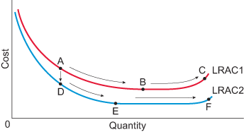
This diagram has ‘Cost’ on the vertical axis and ‘Quantity’ on the horizontal axis.

It shows two very shallow U shaped curves, one just above the other. The upper curve is labelled ‘LRAC1’. The lower curve is labelled ‘LRAC2’. The lowest sections of both curves are actually quite flat for a long section before rising again. The upward rising section of both curves is very short.

Three points are marked on LRAC1. Point A is marked about half way along the downward sloping section of the curve. Point B is marked at the lowest point of the curve. Point C is marked on the upward rising section of the curve.

Three points are also marked on LRAC2. Point D is marked about half way along the downward sloping section of the curve. Point D lies directly below point A on LRAC1. Back on LRAC2, Point E is marked at the start of the flat lowest part of the curve. Point F is marked on the upward rising section of the curve.

Figure 29 Two LRAC curves

A firm moving from point A to B is a clear example of economies of scale: average cost falls as output increases. If the firm were on LRAC 2, then moving from D to E would also be an example of economies of scale.

Note that learning by doing cannot be shown on Figure 30. All LRACs (like the curve used above) show output for a given period of time on the horizontal axis. However, learning by doing is gained from cumulative experience of production, which is gained over time, not necessarily as a result of increasing output per day or per year.

From point A to point D, the firm’s LRAC has shifted downwards, so it is an example of technological change. Note in this example, at any output the firm’s average cost is lower having shifted to LRAC 2 compared to LRAC 1.

Diseconomies of scale only occur when a firm experiences increases to average cost as output rises. This occurs on LRAC 1 as the firm moves from B to C, and on LRAC 2 as the firm moves from E to F.

Each of the LRAC curves shown have a point which identified the minimum efficient scale (MES). For LRAC 1, this is point B, and for LRAC 2, this is point E. The MES occurs at the lowest level of output where average cost is at a minimum.

Economies of scale

Sources of economies of scale can be divided into different types. These types relate to how the activities of the firm are organised in order to reduce the average cost of production as output increases. Broadly, there are three sources of internal economies of scale; two you have met already: economies of increased dimensions, and specialisation. Now we will introduce one more: indivisibilities.

Types of economies of scale (1)

Here is a quick description of three sources of internal economies of scale:

• Specialisation. As the output of the firm increases, each worker can become more specialised in discrete parts of the production process. As each worker becomes more specialised, their efficiency increases.
• Economies of increased dimensions. As output increases, the firm will need to increase the capacity of storage, transport or production space. As the result of a simple geometric relationship, doubling the dimensions of a warehouse will result in a greater than doubling increase to capacity. The capacity of the firm will increase more rapidly than the costs of increasing the dimensions. This can also mean it is better for a firm to bring production to a single location, as increasing dimensions of an existing production facility may be more efficient than having two separate (and smaller) production sites.
• Indivisibility. This occurs when a firm requires a minimum amount of input to operate, and as output increases, the cost of any inputs can be spread over a greater output. As a result, average cost falls as output increases. For instance, consider a steel works: making steel involves using a blast furnace, which has a big cost whether a small or large amount of steel is produced. A furnace is not divisible, so economies of scale are gained when output is increased and the furnace is used more efficiently.

Types of economies of scale (2)

Activity 20

Read each case study below and then, by dragging the labels, match each case study to the correct type of internal economy of scale.

Figure 30 Example A: An oil firm upgrades its transport fleet to bigger tankers.

Figure 31 Example B: A small firm decides to pursue a strategy of innovation to increase output. Initially, the R&D budget comprises the majority of the firm’s total costs.

Figure 32 Example C: A white goods manufacturer organises staff into production teams responsible for different stages of production and assembly.

Increased dimensions

Example A

Indivisibility

Example B

Specialisation

Example C

Using the following two lists, match each numbered item with the correct letter.

1. Increased dimensions

2. Indivisibility

3. Specialisation

• a.Example C

• b.Example B

• c.Example A

The correct answers are:

• 1 = c
• 2 = b
• 3 = a

Answer

Example A is a case of economies of increased dimensions because of the geometric relationship between volume and surface area. For instance, consider two tanker ships: the first a ‘coastal tanker’, 200 m long, 30 m wide and 16 m deep; the second an ultra large crude carrier (ULCC) with dimensions double the length: 400 m long, 60 m wide and 30 m deep. The volume (length × width × depth), increases from 96 000 to 720 000 cubic meters. A doubling of dimensions would increase the cost of construction, however, the volume of goods that can be transported has increased by a factor of more than seven. If the firm can increase its output to fill larger and larger carriers, then the average cost of transport falls.

Figure 33

Example B is a case of indivisibility. Investment in R&D is considered indivisible because it requires significant investment to yield results, and it is difficult to operate R&D below a minimum scale. As output increases, the costs of doing R&D are spread over a greater output, so average cost falls.

Example C is a case of specialisation. At Miele, the washing machine production process is divided into different stages. Workers train on particular stages, for instance, some are forklift drivers and some are engineers making sure equipment operates efficiently. Others focus on stages in the final assembly, checking different components of washing machines and distribution of goods. This type of specialisation would be expected to reduce average cost as the firm’s output increases. As output increases, workers can become more and more specialised, and so the efficiency of the production process increases and results in falling average cost.

Costs in the short run

The previous activities in this section have examined LRAC curves. Now we will look at short run average cost (SRAC) curves.

In the short run, the firm can only change output by changing variable factors. It has to make do with existing fixed factors. This reduces the opportunity to reduce average cost as output increases. In fact, in the short run, average cost is likely to rise once output reaches a certain level. The next set of activities will help you to understand the main features of the SRAC.

Short run average cost (SRAC) curves (1)

Short run average cost (SRAC) curves (2)

It’s often easier to represent cost curves graphically. Here the two columns of data in Table 4 are shown in separate graphs. The table is repeated below.

Figure 34 Total cost and average cost curves

Show description|Hide description

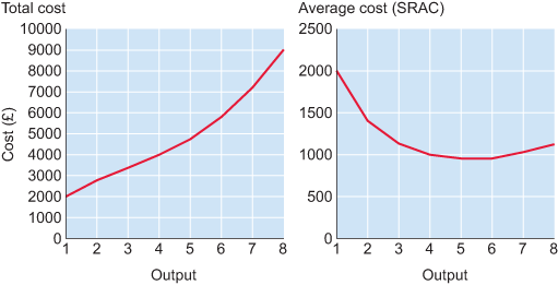
This figure shows two graphs side by side.

Both have ‘Cost (£)’ on the vertical axis and ‘Output’ on the horizontal axis. Both output axes run from 1 to 8 but the vertical axes have different scales. The graph on the left runs from zero up to 10,000 in intervals of 1000. The graph on the right runs from zero to 2,500 in intervals of 500.

These graphs plot the data in the table.

The left graph shows a line rising steadily upwards from a plot of output1, £2000, (which is a point on the vertical axis) up to a plot of output 8,£9000.

The right graph shows a very shallow U shaped curve, starting at a plot of Output 1,£2000, (which is a point on the vertical axis), steadily falling to a minimum point on the curve of Output 5,£950 and then a very gentle rise to Output 8, £1125.

Figure 34 Total cost and average cost curves

Notice that total cost increases with output, albeit at varying rates. The SRAC captures how average cost (or unit cost) changes with output. When output is low, initially average cost falls, but as output increases, average cost starts to rise. Next let’s examine the components of average cost – fixed and variable cost.

Fixed and variable costs

In the short run, some of the firm’s costs are fixed – these are costs that do not change with output. The remaining costs are variable – they change with the level of output.

The following video will help you to work through the difference between fixed and variable costs, and also show how we can apply these concepts to the SRAC curve.

Watch the video and then attempt Activity 22.

Download this video clip.Video player: Fixed and variable cost

Show transcript|Hide transcript

Transcript: Fixed and variable cost

SPEAKER

Let's consider a firm supplying tablet computers. The firm produces tablets in-house. The capital and land needed for production at the firm include an administrative head office and a manufacturing site. These are fixed factors of production-- in the short-run, they cannot be changed. After all, it takes time to expand buildings and develop new production facilities.

Let's assume the firm pays an annual rental charge for the use of buildings and machinery. In the short-run, the firm's fixed factors represent a fixed cost. A fixed cost does not change with output. But the firm can squeeze more staff into its existing buildings to help increase output without altering the size of buildings or the amount of equipment.

The firm can produce more tablet computers by increasing its use of variable factors, such as labor and raw materials. Increasing output will mean more work needs to be done. Additional forklift truck drivers will be needed to move raw materials. Similarly, more engineers will be needed to service equipment and provide adequate maintenance. More administrative staff will be required in the head office to manage the increasing flow of labour. And, of course, the amount of raw materials used will also increase.

If the firm increases its variable inputs, output will increase. In the short-run, the variable costs will increase while our fixed costs remain unchanged. Fixed cost is constant-- it's the same at all levels of output, so it's represented by a horizontal straight line on the diagram. Here we are showing costs on the vertical axis, and quantity produced per week on the horizontal axis.

But average fixed cost will change as output increases. Average fixed cost must fall as output rises. As output is increased, the fixed cost is spread over larger and larger numbers of units. The average fixed cost will get smaller and smaller. So the average fixed cost curve looks like this.

Variable costs increase with output. If we assume that this firm experiences increasing returns to variable factors at low levels of output and decreasing returns at high output, then we can draw an average variable cost curve which has a U shape. Now we have a U shape cost curve for average variable cost, and a cost curve for average fixed cost. Now we can add these two curves together to produce an average total cost curve which we'll label AC for our average cost curve.

Since we're adding together two cost curves, we must sum vertically. Average fixed cost plus average variable cost gives average total cost, more simply called average cost. So at Q1, average variable cost is equal to AVC1, to which we add the average fixed cost AFC1 to give a value of average cost, AC1. AVC1 plus AFC1 equals AC1.

Now we have one point on the firm's average cost curve. Similarly, for Q2 we have AVC2 plus AFC2 equals AC2. The same reasoning applies for Q3 and Q4. So we can repeat this process for all possible levels of output and so derive the average cost curve.

At low levels of output, average cost is falling. This is because, firstly, average fixed cost falls as output is increased. And secondly, average variable cost fall due to increasing returns to the variable factors being used by the firm.

At higher output levels, average variable cost rises due to the effect of diminishing returns to the variable factors which outweigh the decrease in average fixed cost. The average cost curve takes the shape of a U, falling as output is increased when output is low, and rising as output continues to be increased at high output levels. Because economists expect that the same kind of thing will happen in all, or at least most, production processes, the U-shaped average cost curve is the model that economists use in analysing the short-run behaviour of firms' costs.

End transcript: Fixed and variable cost

Download

Fixed and variable cost

Short run cost curves (1)

Activity 22

In the figure below we have an average (total) cost curve, an average fixed cost curve and an average variable cost curve. Using the drag and drop boxes, label the graph correctly.

Active content not displayed. This content requires JavaScript to be enabled.

Figure 35 Short run average cost curves (1)

Interactive feature not available in single page view (see it in standard view).

Answer

The correctly labelled figure is shown below.

Figure 36

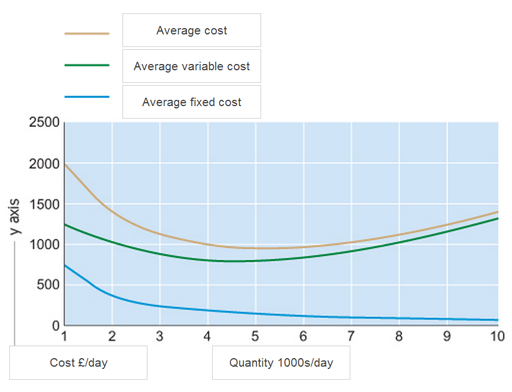
The cost curve has a vertical axis showing the cost in £ per unit. The horizontal axis shows the quantity, or units produced per day. This is shown in thousands of units per day.

The figure shows three short run cost curves.

• The lowest curve shows average fixed cost; average fixed cost will always fall as output increases.
• Next average variable cost; average variable cost has a characteristic ‘u’ shape due to the increasing and diminishing returns to variable factors.
• Finally, the average cost curve (sometimes referred to as average total cost curve) is the sum of average fixed and average variable cost. This means average cost is always greater than average variable or average fixed cost.

Notice that as output increases, the difference between average cost and average variable cost reduces. This is because average fixed cost decreases with output. Another way to think about it is that the difference between average cost and average variable cost equals average fixed cost.

Short run cost curves (2)

The next activity will check that you can interpret the shape of the average cost, average variable and average fixed cost curves described in the video, Fixed and variable cost.

Activity 23a

Click on the short run cost curve figure below to identify the approximate point where average costs are at a minimum.

Active content not displayed. This content requires JavaScript to be enabled.

Figure 37 Average cost curves (2)

Interactive feature not available in single page view (see it in standard view).

Discussion

Look at the figure below. The red arrow shows the correct answer for the point of minimum average cost.

The brown arrow shows the point of minimum average variable cost. The average fixed cost curve has no minimum as it decreases with every unit of output (it is not u-shaped).

Figure 38

Show description|Hide description

This diagram has ‘Cost £s per day’ on the vertical axis, which is marked from zero to 2500, in intervals of 500.

The horizontal axis is labelled ‘Quantity, thousands per day’ and this is marked from zero on the left up to 10 on the right.

Three curves are shown, one above the other. The upper curve is labelled ‘AC’. AC starts at a plot of 1000 Quantity, 2000 Cost. The curve slopes down steeply at first before gradually getting shallower to reach a minimum point at just over 5000 Quantity, 900 Cost. The curve then rises gradually.

The middle of the three curves lies below AC and is labelled ‘AVC’. AVC starts at a plot of 1000 Quantity, 1250 Cost. Its downward slope is shallower than AC and it reaches its minimum point at 4500 Quantity, 800 Cost. The curve then rises, with almost the same upward slope as the AC curve. It very gradually runs closer to the AC curve that lies just above it.

The lower curve is labelled ‘AFC’. AFC starts at a plot 1000 Quantity, 750 Cost. This curve slopes steeply down initially for a very short distance but it then becomes almost flat, with a very shallow downward slope. The curve ends just above the horizontal axis.

Two vertical upward arrows are shown, both running from the horizontal axis, a red one up to the minimum point of the AVC curve and a green one up to the minimum point of the AC curve.

Figure 38

Short run cost curves (3)

Activity 23b

This time, click on the quantity axis in the figure to identify the level output where the difference between average cost and average variable cost is smallest.

Active content not displayed. This content requires JavaScript to be enabled.

Figure 39 Average cost curves (3)

Interactive feature not available in single page view (see it in standard view).

Discussion

The difference between average cost (AC) and average variable cost (AVC) is least when output is high, in this case at a quantity of 10 000/day (see the black arrow on the figure below). This is the same as spotting that average fixed costs (AFC) are lowest when output is high, because: AC – AVC = AFC. In the short run, if output were to continue to increase beyond a quantity of 10 000/day then we would expect AFC to become smaller and smaller, and so make a smaller and smaller contribution to AC.

Figure 40

Show description|Hide description

This diagram shows the same curves as the previous diagram. It has ‘Cost £s per day’ on the vertical axis, and it is marked from zero to 2500, at intervals of 500.

The horizontal axis is labelled ‘Quantity, thousands per day’ and this is marked from zero on the left up to 10 on the right, at intervals of one.

Three curves are shown, one above the other. The upper curve is labelled ‘AC’. AC starts at a plot of 1000 Quantity, 2000 Cost. The curve slopes down steeply at first before gradually getting shallower to reach a minimum point at just over 5000 Quantity, 900 Cost. The curve then rises gradually.

The middle of the curves lies below AC and is labelled ‘AVC’. AVC starts at a plot of 1000 Quantity, 1250 Cost. Its downward slope is shallower than AC and it reaches its minimum point at 4500 Quantity, 800 Cost. The curve then rises, with almost the same upward slope as the AC curve. It very gradually runs closer to the AC curve that lies just above it.

The lower curve is labelled ‘AFC’. AFC starts at a plot 1000 Quantity, 750 Cost. This curve slopes steeply down initially for a very short distance but it then becomes almost flat, with a very shallow downward slope. The curve ends just above the horizontal axis.

On this diagram, one vertical upward black arrow is shown, running from the end of the horizontal axis at output 10,000 up to the AVC curve.

Figure 40

Short run cost curves (4)

Activity 23c

Select the answer for

Activity 23c

here

If output is at a quantity of 3000 per day, using the figure below, pick one answer describing how the average cost will change if output is increased to 3001 per day.

Figure 41 Average cost curves (4)

Show description|Hide description

This diagram is exactly the same as the previous figure. It has ‘Cost £s per day’ on the vertical axis, and it is marked from zero to 2500, at intervals of 500.

The horizontal axis is labelled ‘Quantity, thousands per day’ and this is marked from zero on the left up to 10 on the right, at intervals of one.

Three curves are shown, one above the other. The upper curve is labelled ‘AC’. AC starts at a plot of 1000 Quantity, 2000 Cost. The curve slopes down steeply at first before gradually getting shallower to reach a minimum point at just over 5000 Quantity, 900 Cost. The curve then rises gradually.

The middle of the curves lies below AC and is labelled ‘AVC’. AVC starts at a plot of 1000 Quantity, 1250 Cost. Its downward slope is shallower than AC and it reaches its minimum point at 4500 Quantity, 800 Cost. The curve then rises, with almost the same upward slope as the AC curve. It very gradually runs closer to the AC curve that lies just above it.

The lower curve is labelled ‘AFC’. AFC starts at a plot 1000 Quantity, 750 Cost. This curve slopes steeply down initially for a very short distance but it then becomes almost flat, with a very shallow downward slope. The curve ends just above the horizontal axis.

On this diagram, one vertical upward black arrow is shown, running from the end of the horizontal axis at output 10,000 up to the AVC curve.

Figure 41 Average cost curves (4)

Increase

Decrease

Remain unchanged

 

a. 

Increase

b. 

Decrease

c. 

Remain unchanged

The correct answer is b.

Answer

If output increases from a quantity of 3000 per day, average cost will fall. This is because at this output the average cost curve is sloping downwards.

Increasing output will reduce the average cost until it reaches a minimum at a quantity of approximately 5000 per day. Then the average cost curve slopes upwards, so average cost increases when output increases beyond 5000 per day.

Cost curve summary

This section has highlighted some important properties of cost curves. Because we expect the behaviour of costs to be similar in most firms and for most production processes, we have a model of firms’ costs that we can apply widely.

In the long run the firm can:

• vary all inputs to minimise cost
• reduce average cost by:
  • adopting new technologies
  • increasing output to gain from economies of scale
  • over time, reducing average cost from learning by doing
• achieve no further cost saving advantages from increasing output once output is at MES.

In the short run:

• the firm is expected to have a u-shaped average cost curve
• the average cost curve shows how costs change at different levels of output
• average cost is the sum of the average fixed cost and average variable cost
• average fixed costs decrease as output increases
• average variable costs have a u-shaped curve because of the returns to inputs of variable factors vary with output
• at low levels of output, a firm is expected to experience increasing returns to variable factors, and at higher levels of output there will be diminishing returns.

The u shape of the short run average cost curve also implies something about the marginal cost curve, which we look at next.

7.5 Marginal cost curves

Now you have learned the properties of the average cost curve, you will check your understanding of marginal cost. Average cost and marginal cost are fundamental economic concepts in the analysis of how firms, industries and markets behave.

Average cost and marginal costs (1)

Watch the short video on marginal cost, which describes the relationship between average and marginal costs. Make sure you understand the difference between average and marginal costs.

Download this video clip.Video player: Marginal cost

Show transcript|Hide transcript

Transcript: Marginal cost

INSTRUCTOR

Activities this week have already discussed in detail the concept of average cost and the average cost curve. Another measure of cost is marginal cost. Marginal cost is the change in total cost incurred as a result of producing an extra unit of output. Marginal cost and average cost are closely related.

To see how marginal cost and average cost are related, let's think about the average height of people in a room. Consider how the average height changes when an extra person enters. For instance, if the room contains just three people, we can calculate the average height of people in the room.

Suppose a fourth person enters. We can call this extra person the marginal person. If the marginal person is shorter than the average height of people already in the room, then the average height of people will fall. We can use the same idea to look at what happens to average cost in a firm when an additional unit of output is produced.

Let's consider a typical average cost curve for a firm. If average cost is falling as a firm increases its quantity of output, then the cost of each marginal unit of output must be less than the average cost. For instance, at output Q1, the marginal cost must be less than the average cost. The marginal cost, the cost of producing an additional unit, lies below the average cost curve.

When average cost is rising as output increases, then marginal cost must be greater than average cost. For instance, at output Q2, the marginal cost must be above the average cost curve. With every additional unit of output, average cost increases. Marginal cost is greater than average cost.

Average cost and marginal cost are only equal when average cost is no longer falling, and has not started to rise. In other words, average cost is at a minimum. Average cost is at a minimum when output is Q3.

As a quantity less than Q3, marginal cost is less than average cost. Marginal cost can be drawn as a curve like this. To the right of Q3, marginal cost is greater than average cost, and the marginal cost curve is drawn like this. The marginal cost curve intersects the average cost curve where average cost is at a minimum.

Now we have described the marginal cost curve whose shape and position are determined by the shape of the average cost curve. As we will see later in the block, economists use marginal cost to analyse firms' decisions about how much output to produce.

End transcript: Marginal cost

Download

Marginal cost

Average cost and marginal costs (2)

Calculating marginal cost

So far we have analysed the relationship between average cost and marginal cost. This activity will check that you can calculate marginal cost.

7.6 Using evidence

This section is an opportunity to practise relating some of the theory of production cost to help you analyse production activities in firms.

Cost of producing a pint

Producing a pint of milk is a costly business. Firms producing milk, usually referred to as dairy farms, take inputs in the form of land, capital (the herd, milking parlours and storage) and raw materials (such as feed and seed). They then use these inputs to make milk, which can also be used to produce cheese and yogurt.

Activity 26

Some farms may receive income from the government, but like all firms, if their income doesn’t cover the cost of milk production, they risk going out of business. Watch this short video on the challenges facing milk producers, which introduces one of the main ideas covered in Section 7: reducing cost. Notice how the video uses ideas from short run and long run cost curves.

Whilst watching the video, think about the key challenges milk producers face and what they can do to reduce these challenges. Make some notes on your thoughts here – you will need to refer back to them later on.

Download this video clip.Video player: Costs of milk production

Show transcript|Hide transcript

Transcript: Costs of milk production

JOHN CRAVEN

The auction's going well, with strong interest in Ken's herd. The price farmers get for their milk is the highest for 15 years, but the average dairy farmer's profit margin is being squeezed by spiralling costs.

A pint of milk costs us consumers about 48 pence. Now, of that, 15 pence goes to the farmers. The rest of it goes to the processors and to the retailers.

Now, what about the farmers' costs? Well, of that 15 pence, 9 pence goes on to variable costs - things like feed and vet's bills, bedding, fertilisers and those sort of things. Then there's another 6 pence going to overhead costs, such as fuel, electricity and, of course, wages.

And that's it. The bottle's empty. The farmer has broken even. But that doesn't take into account his extra costs, such as depreciation, and vital investment in the future. When you add that on, the farmer is losing at least one penny for every pint.

Dairy farmers like Ken say they aren't asking for the earth. Just a little more a litre would make all the difference.

Vicky, you were Ken's milk buyer. A lot of people will say, well, look. We pay 48 pence a pint for our milk, and the farmer's only getting 15 pence. People like yourself are getting an unfair share.

VICKY HICKS

Well, I mean, I think figures recently published by Dairyco themselves actually show that the biggest proportion in the supply chain has actually gone to the supermarkets. They do relatively little, and actually get relatively a lot for what they do. All they do is put the milk on the shelves. We have to process it and pack it, and that itself is a very small margin to what we have to work to to sell it to the supermarkets, or whoever our customers may be. And they dictate what we can pay.

JOHN CRAVEN

There are around 11,000 dairy farms in England and Wales. That's half what there were 20 years ago. But every day for the past 12 months, two dairy farms have closed. That keeps auctioneers like Gwilym Richards busy.

Dairy farmers are facing a crisis. Rising costs mean many are losing money on every pint of milk they produce. Rather than give up on dairy, others see a supersized future. In America, the mega-dairy is already a reality. This is just a small part of a 30,000 cow farm in Indiana.

In Gloucestershire, David Ball has 750 cows. Only by getting bigger has he been able to turn the white stuff into a profit.

Well, you've put a huge investment into things like the milking machines here.

DAVID BALL

That's right. I mean, this equipment represents a huge capital investment.

JOHN CRAVEN

How much, roughly?

DAVID BALL

So this would be in excess of 200,000 pounds for this milking equipment. And so, therefore, we need to use it as efficiently as we possibly can. And if that means putting more cows through it in order to utilise it more efficiently, then it represents a better return on that investment.

JOHN CRAVEN

So how many times do your cows get milked every day?

DAVID BALL

The cows come through here three times a day, and the equipment will be running for 15 to 18 hours a day.

JOHN CRAVEN

So it's really earning its keep

DAVID BALL

Indeed, yes.

JOHN CRAVEN

David's herd is one of Britain's biggest. But could mega-dairies be the ultimate answer?

PRESENTER

The scale of this farming operation is absolutely enormous. I've never seen anything like it in my life. Each of these sheds has got about 3000 cows in it, and there's ten units spread out across this farm.

And you can't see any of the cows because they're all indoors. They never go outside. It makes my farm look like an allotment.

JOHN CRAVEN

Adam, obviously taken aback by the size of that farm, David. And you've been to that very same place. Is it the way that UK dairy farming will go eventually?

DAVID BALL

I think that the scale that we've seen there represents a huge step forward from where we are here, and so that will be a long time before we see anything of that nature here. But generally speaking, over time, sizes of businesses grow.

JOHN CRAVEN

But not to thirty-odd thousand cows, you don't think?

DAVID BALL

I don't think that's going to happen here, because we haven't got the space.

JOHN CRAVEN

We might never see the scale of the American mega-dairy in the UK. But while some smaller dairy farms decide to call it a day, those that want to carry on are finding that getting bigger is the only way to survive. Bigger may be better for business, but will we, the consumer, be happy with the idea of huge herds living 24 hours a day indoors rather than in fields?

End transcript: Costs of milk production

Download

Costs of milk production

Interactive feature not available in single page view (see it in standard view).

To use this interactive functionality a free OU account is required. Sign in or register.

Interactive feature not available in single page view (see it in standard view).

Discussion

Here are some notes about the video – you may have some similar points in your notes.

• Costs of production are high, sometimes higher than the price dairy farmers are paid, and rising.
• Milk prices are falling.
• Farmers have difficulty investing in new equipment to replace worn or old equipment – this wear and tear cost is what the presenter, John Craven, refers to as ‘depreciation cost’.
• Some producers are considering stopping milk production.

Possible responses to reduce cost:

• Invest in new technology to shift the farm’s long run cost curve downwards, for example, by buying more equipment that is more efficient to run, or updating their production process (production function) to reduce labour input. However, this is difficult if the farmer cannot afford to increase their fixed cost in the short run to purchase new equipment.
• Gain from economies of scale by increasing their scale of output, like in the mega dairy example. If firms invest in new technology, not only may they experience a downward shift in the LRAC, they may also benefit from decreasing unit cost as output increases. This may be as a result of economies of scale arising from indivisibility – that costs per unit of output from running and maintaining new technology or machinery will decrease as output increases. Other indivisibilities may arise from the running of the farm office and administration, which have a fixed cost whether the farm has a high or low output, but if spread over higher output, will help to decrease average cost.
• Stop producing milk.

Challenges:

• Most farms are small in the UK, and land is scarce and expensive. It may not be easy to increase the scale of the business, like in the mega dairy example.
• Some overseas producers already produce at a lower cost per pint.
• Economies of scale require investment in production, which is difficult when making a loss.
• Issues of animal welfare related to the mega dairy.

Labour and fixed cost

Did you notice anything peculiar about the analysis of labour cost in the video? Try Activity 27 to test your understanding.

Cost of inputs

In 2012, farmers argued that income received for milk fell below the cost of production. The video clip suggests part of the reason for this is due to rising input costs in dairy production. The next activity presents some data on dairy costs, which can be analysed to see if this supports the material given in the clip.

Activity 28

Look at the data table below, which shows an extract from the National Farmers’ Union (NFU) 2011 report on dairy production cost. There is also a time series chart showing the monthly price of feed cost, given in pence per litre of milk, in the years leading up to 2012.

Does the data below support the view of farmers in the video?

Extract from NFU (2011) Report. Fixed and variable cost of dairy production (Source: DairyCo. 2012a)

Figure 44 Dairy production costs data

Source: DairyCo. 2012a, author calculation

Figure 45 Total feed cost in pence per litre (ppl) of milk produced over time, shown in red with a linear trend line shown in black

To use this interactive functionality a free OU account is required. Sign in or register.

Interactive feature not available in single page view (see it in standard view).

Discussion

Here are some notes made on the Dairy Co. (2012a) and NFU (2011) data:

The NFU (2011) table reports data for two years: 2009/10 and 2010/11. It reports that total costs have increased 6 per cent over the two years. Notice that the costs are given per litre – effectively this is average cost data – average cost per litre. Notably the rise in cost is due to variable costs having risen by 11 per cent between 2009/10 and 2010/11, whilst fixed costs have only risen by 0.5 per cent.

In particular, the cost of variable inputs per pint, such as fertilisers and veterinary costs, show rises between 2009/10 and 2010/11. This would seem to support that profits (margin) in dairy are being squeezed – prices are falling whilst costs are rising. However, we have to be cautious – this is only one year of data – it could be a one-off or ‘outlier’ year. In the short run, if dairy producers increased output, then average variable cost could rise as a result of diminishing returns.

The graph using DairyCo. (2012a) data shows some data on feed cost – a raw material for dairy producers. This seems partially to support the NFU report – the linear trend, as shown by the black line, shows variable costs, such as feed costs, rise on average over time. For instance, the price of feed in 2004 ranges from approximately 3 ppl to 4.5 ppl, compared to a range of 5.5 ppl to 8.5 ppl in 2011. However, although the trend is for increasing prices, the chart also shows considerable variability in the cost of feed within each year, possibly due to seasonal changes in the cost of feed.

There seems to be evidence that variable costs are rising. However, notice that we have no data on how fixed costs are changing over time.

Profits and cost

The evidence in this section suggests milk producers are relatively helpless: dairy producer profit per litre is declining as costs rise and milk prices fall. However, not everyone agrees with this view.

DairyCo., a division of the Agriculture and Horticulture Development Board (AHDB) responsible for making UK agriculture competitive and sustainable, produced a report in 2012 which looked at factors that influenced producers’ margins (profits). It found a significant variation in the production cost per litre of different firms. Some firms could produce milk more efficiently than others. The report stated that:

The report also concludes:

7.7 Summary

Section 7 has examined the firm and, in particular, different measures of cost. It has looked at costs in the short run and the long run. It has shown how firms might reduce average cost in the long run, and the constraints that firms face in the short run. You have worked through activities using cost curves to show how average costs are related to output in a period (e.g. per day or week). Understanding cost curves is key to understanding the behaviour of firms, industries, markets, and more widely, the supply side of the economy.

8 Conclusion

In this OpenLearn course you have developed your understanding of how economists use models by exploring the construction and use of macroeconomic models to analyse the determination of income, and by seeing how the microeconomic analysis of firms adds yet another dimension to what economists do.

In Section 1, you were introduced to the founder of macroeconomics, John Maynard Keynes.

In Section 2, you learnt how the circular flow model can be used to show either actual or planned values of economic variables. In connection with this, you considered the difference between an identity (as used in the national income accounting system) and an equality (as used in the Keynesian theory of national income equilibrium).

In Section 3, you built up a Keynesian consumption function from its components of exogenous consumption and income-induced consumption, making use of the concept of the marginal propensity to consume.

In Section 4, you looked at the modelling of saving and investment, noting how investment and consumption together make up aggregate demand in the model of a closed economy with no government sector. You also learnt about the importance of the 45-degree line in analysing equilibrium.

In Section 5, you considered how equilibrium may occur at below full employment and how full employment may be achieved by a stimulus to aggregate demand. The macroeconomic analysis ended with Section 6, which showed you how fiscal policy can be used to stimulate demand, and taught you about the importance Keynes placed on the role of the government in leading economies to better outcomes.

Section 7 concluded the course by zooming in on firms and examining some of the major factors that determine their viability and competitiveness.

References

Acknowledgements

Except for third party materials and otherwise stated (see terms and conditions), this content is made available under a Creative Commons Attribution-NonCommercial-ShareAlike 4.0 Licence.

The material acknowledged below is Proprietary and used under licence (not subject to Creative Commons Licence). Grateful acknowledgement is made to the following sources for permission to reproduce material in this free course:

Every effort has been made to contact copyright owners. If any have been inadvertently overlooked, the publishers will be pleased to make the necessary arrangements at the first opportunity.

Course image: Enrique Jiménez in Flickr made available under Creative Commons Attribution-NonCommercial-ShareAlike 2.0 Licence.

Don't miss out

If reading this text has inspired you to learn more, you may be interested in joining the millions of people who discover our free learning resources and qualifications by visiting The Open University – www.open.edu/ openlearn/ free-courses.