Innovation, markets and industrial change
Use 'Print preview' to check the number of pages and printer settings.
Print functionality varies between browsers.
Printable page generated Tuesday, 9 June 2026, 5:36 AM
Innovation, markets and industrial change
Introduction
This course looks at the role of innovation in the development of industries and considers how production costs change as sales increase and as new technology is introduced into the production process. It looks at the relation between consumer demand for a good and that good's price, and at how the relation between output and production costs in different markets can dramatically affect industry structure. In describing these issues, the course introduces the range of activities that constitutes economics: formulating theories, modelling, debate and persuasion, analysis of data, understanding the behaviour of economic institutions such as companies and households, and analysing economic processes. It also seeks to show how all of these economic techniques can be used to build up a rich understanding of innovation and economic change.
This OpenLearn course provides a sample of Level 1 study in Sociology.
Learning outcomes
After studying this course, you should be able to:
appreciate the importance of technological change, costs of production and consumer preferences to the changing organisation of production
understand the relation between the quantity demanded of a good and its price as represented by the demand curve
understand economic models of the relation between firms’ costs and output
analyse the role of technology and costs in influencing industry structure over the life cycle.
1 Technological change, demand and costs
The new economy
Over the past 40 years global computing power has increased a billionfold. Number-crunching tasks that once took a week can now be done in seconds. Today a Ford Taurus car contains more computing power than the multimillion-dollar mainframe computers used in the Apollo space programme. Cheaper processing allows computers to be used for more and more purposes. In 1985, it cost Ford $60,000 each time it crashed a car into a wall to find out what would happen in an accident. Now a collision can be simulated by computer for around $100. BP Amoco uses 3D seismic-exploration technology to prospect for oil, cutting the cost of finding oil from nearly $10 a barrel in 1991 to only $1 today …
Thanks to rapidly falling prices, computers and the Internet are being adopted more quickly than previous general-purpose technologies, such as steam and electricity. It took more than a century after its invention before steam became the dominant source of power in Britain. Electricity achieved a 50% share of the power used by America's manufacturing industry 90 years after the discovery of electromagnetic induction, and 40 years after the first power station was built. By contrast, half of all Americans already use a personal computer, 50 years after the invention of computers and only 30 years after the microprocessor was invented. The Internet is approaching 50% penetration in America 30 years after it was invented and only seven years since it was launched commercially in 1993.
(The Economist, 23 September 2000, pp. 5, 10)
That is how The Economist discussed the issue of information technology as a general purpose technology.
Question
How would you summarise the argument about prices, costs and information technology put forward in The Economist?
Discussion
It seems to us that the argument is that improvements in information technology caused a decline in the costs that firms face in producing goods. Falling prices have in turn encouraged a rapid take-up by consumers of products embodying information technology. Economists place costs on the supply side of markets, where firms produce and sell goods such as cars, oil, personal computers and Internet access. Take-up by consumers is on the demand side of the market. The quotation suggests that new information technology causes a decline in costs and hence in prices that enables large numbers of consumers to buy safer cars, personal computers and so on. Technological change, a supply-side phenomenon, is seen as a prime cause of economic change.
In D202_2, the author looked at the impact of newly introduced technologies in the early phase of the US auto industry and the PC industry, highlighting the similarities between what we are observing today in the IT-based industries and what we observed 100 years ago in an industry we now consider mature. As we write, technological change continues to be very rapid, and two particular technological developments will be used in this chapter to illustrate our discussion of the forces shaping the organisation of industrial production. The dilemma faced by car manufacturers in adjusting to the hydrogen economy’ of the future will be discussed in Section 4. We also discuss digital technology, which has revolutionised sound reproduction as well as the capture and transmission of visual images in DVD, digital television and digital cameras. Car manufacturers are also exploiting its potential. For example, the Citroën C5 ‘bristles with the latest digital technology to improve your motoring experience’ (see Figure 1). An advertisement for the C5 alludes to the origins of digital technology, showing instructions as sequences of ‘switches’ in a computer as being ‘on’ or ‘off’, or set to ‘1’ or ‘0’.

In this course we will introduce the use of economic models of markets, firms and industries to examine the relationships among consumer demand, technological change and costs. Section 2 develops the idea expressed in The Economist extract that falling prices were responsible for the rapid take-up of new products by consumers. This is an example of a widely observed relation between the quantity demanded of a good by consumers and the price of the good: the lower the price, the greater the quantity demanded. However, there are other influences on market demand. For example, consumers are likely to buy more goods if their incomes increase. So Section 2 explains how economists analyse the interaction between price and other influences. This analysis is the first part of the theory of consumer demand.
The rest of the course focuses mainly on the supply side of the market, exploring the role of costs and technological change in the organisation of production. The objective is to understand the process by which a firm – initially one among many similar firms jostling for position – emerges ahead of the pack to achieve an advantage over its competitors, as Ford did in the US automobile industry. What was so special about Ford? More generally, how can we account for the change in structure that so many industries seem to undergo? Why do most of the many small firms so common in the early years of new industries disappear to leave an established industry dominated by a few large firms? Why does the heterogeneity or extreme variety of those small firms in new industries give way to a much greater degree of similarity, indeed standardisation, among the few survivors?
In exploring these questions, economists use models of the relation between the output, technology and costs of firms. In Section 3, we define technology in an economic model of a firm, and use it to explore the link between technology and costs. We begin from a model in which firms take technology as given and their ability to change their costs is severely constrained, and then build in progressively more decision-making flexibility over the adoption and use of technology.
Section 4 links this analysis of technology and costs to the model of the industry ‘life cycle’ introduced in DD202_2. The life-cycle model represents an industry as if it were a biological organism going through the stages of birth, growth, maturity and decline, and is used to consider the interaction of demand and technology in shaping industrial structure. This section further extends the analysis of firms, technology and costs to include models where firms’ freedom to learn and create is one driver of technological change itself. This helps us to understand how a particular firm can become the ‘leader of the pack’ through innovation and how it can then gain an advantage over competitors by reducing its costs through large-scale production.
2 Market demand
2.1 Industry and markets: what do we mean?
Case study: Digital outsells film
Sales of digital cameras have overtaken traditional 35 mm cameras for the first time. According to monthly figures collated by national electric and photo retailer Dixons, digital camera sales outstripped 35 mm cameras during the month of April. ‘This is a sea change in consumer photography,’ said Dixons marketing director Ian Ditcham. ‘As a leading photographic retailer, Dixons is a clear barometer of consumer trends,’ he said. The main reasons for the popularity of digital cameras are falling prices, the growth of home PC and internet usage and the instant delivery of images without the need for processing.
(Adapted from Outdoor Photography, August 2001, no. 15, p. 4)
Questions
What do you think are the main similarities between the arguments in this case study and the second paragraph of ‘The new economy’ quotation discussed in Section 1?
Figure 2 illustrates a number of different makes of digital camera. What other products do you normally associate with the manufacturers of these cameras?

The quotation and the case study describe the take-up by consumers of new products embodying innovations in information technology. Both link the popularity of new technology among consumers with falling prices and draw attention to the rapidity of consumer take-up. There is something new for Dixons and other retailers to sell and for consumers to buy. A new product, the digital camera, has created a new market. Figure 2 shows that this market is supplied by a number of manufacturers normally associated with the production of a range of other consumer goods. Nikon and Olympus make traditional cameras. Epson is a well-known brand of personal computers and printers. Sony is probably best known for the Walkman, the first personal audio-cassette player. Casio puts its name on watches and calculators. Fuji is particularly interesting as a manufacturer not only of cameras but also of film, the medium under challenge from digital.
It seems natural to us to say that these firms from different industries, including computers, electronics and optical equipment, have together created a new market, that is, a market for a new product, the digital camera. (An industry is a group of firms producing a broadly related range of goods using similar technologies. A market is constituted by the buying and selling of goods or services.) In other words, industries can be thought of as being about the production of a range of broadly related goods, and markets are about the sale and purchase of a more narrowly defined set of goods. For example, the optical equipment industry produces cameras, photocopiers, microscopes, telescopes and so on in order to supply different markets. There are consumer markets for disposable cameras, entry-level compact cameras or cameras for the serious amateur and so on. There are industrial markets for cameras for professionals or microscopes for specialist use in medical and scientific research. So markets can be identified in terms of their consumers and the purposes for which those consumers are buying goods, as well as in the more familiar terms of the goods themselves. Phrases such as ‘the market for medium format cameras’ are common. But a medium format camera might appeal to the serious, and affluent, amateur as well as the professional. It is not easy to say where one market ends and another begins.
Precisely where we draw the line between ‘industry’ and ‘market’ depends on which aspect of economic activity we want to analyse. Producing and selling are both stages in a single complex process of making profits from the supply of goods by turning inputs into outputs that consumers are willing and able to buy. It is helpful to use the term ‘industry’ if we want to direct attention towards suppliers (as producers) and the technologies they are using. Most countries use a system known as the Standard Industrial Classification to assign organisations to industries. Under this system, each organisation is assigned to an industrial category according to the principal goods or services it produces. The system is essential to the collection of statistics that enable us to estimate the relative contributions of the different industries to national income, and to detect which parts of the economy are growing or contracting over time.
To speak of a market directs attention towards the relations between suppliers (as sellers) and buyers of a particular good. It is usually taken for granted that buyers and sellers are engaged in voluntary exchange, of money for goods, and that buyers are able to exercise choice (to buy or not to buy, to buy this good rather than that one). ‘Market’ is therefore a politically charged term, unlike ‘industry’, shown, for example, by the prevalence in political debate of the expression ‘free market’.
The focus in Section 2 will be on consumer demand for products and in particular the price at which they are offered for sale. It is therefore appropriate to use the term ‘market’ in this section, reserving ‘industry’ for later sections where our attention is directed towards the costs incurred by firms in producing goods.
2.2 Market demand and price
This subsection will explore the widely observed relationship between the quantity demanded of a good by consumers and the price of the good: the lower the price, the greater the quantity demanded. This relationship underlies the way in which falling prices are responsible for the rapid take-up of new products by consumers, as reported in the quotations above. We focus on the market demand curve, which represents the demand of all the consumers in a given market. However, as well as the price of the good, there are other influences on market demand, discussion of which will be postponed until Section 2.3. This makes it possible to take a step-by-step approach and to begin by considering the influence of price alone.
The relationship between demand and price can be represented in different ways: in words, in a diagram or by using algebra. We expressed it in words in the preceding paragraph: the lower the price, the greater the quantity demanded. This relationship can also be shown in a diagram, known as a demand curve (always by convention a ‘curve’ though it may be drawn as a straight line). Figure 3 shows a demand curve, and we look at it in detail in a moment. Note first that as part of the step-by-step approach, the demand curve is drawn on the assumption that the price of the product is the only relevant variable influencing demand for the product. A ‘variable’ is a precisely defined aspect of the economy, such as the price of a good, that can take a range of values (such as £1, £2, £3,…).
All the other influences on market demand are held constant while we look at the relationship between demand and price. This procedure is usually known by the Latin phrase ceteris paribus, which means ‘other things being equal’. It is the foundation for constructing economic models, which abstract from the complexities of real economic life to concentrate on one or two variables that seem to be important. Once we have understood how two variables are related – how a change in one affects the other, ceteris paribus – it is possible to move on, dropping the assumption that other things have remained equal. We can introduce other variables, gradually making the model more complex by considering the effects of changes in them.
An economic model therefore provides a systematic way of thinking about causal relationships. We can use them to formulate hypotheses about cause and effect, such as ‘lower prices caused the increase in sales’. That puts us in a position to look for evidence that might lead us to accept or reject the hypothesis.
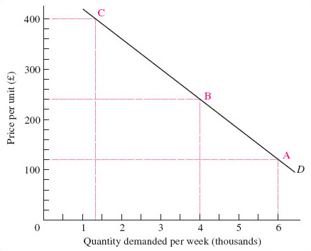
The market demand curve is a very simple economic model in that it abstracts from the many things going on in a market to focus on only two: the quantity demanded of the good and its price. Look at Figure 3, and notice that the vertical and horizontal axes are ‘anchored’ at the zero point, called the origin. As with all such diagrams, movements up the vertical axis, and along the horizontal axis to the right, represent higher values. Each point on the curve D shows the quantity demanded (measured on the horizontal axis) at a particular price (measured on the vertical axis). The market demand curve therefore shows the quantity demanded at each and every price by all the consumers in a particular market. We say ‘each and every price’ to draw attention to the fact that in drawing the market demand curve as a continuous line, economists are making estimates. The good may not have been offered for sale at ‘each and every’ price but only a small number of selected prices. Drawing the market demand curve as a continuous curve on a diagram such as Figure 3 shows estimates of what demand would be at other prices.
Figure 3 shows a hypothetical market demand curve for electronic personal organisers (hypothetical because it is not based on actual sales figures but is being used purely as an illustration of market demand curves in general). Electronic devices are particularly good at storing files, allowing them to be used in different ways, and have come to dominate the market for portable information storage. The market demand curve depicts the quantity consumers demand, depending on price. This ‘quantity demanded’ is not necessarily the number of electronic personal organisers that people need, but what they are willing and able to purchase at different prices.
The demand curve in Figure 3 shows that with a price of £120, the quantity demanded of electronic personal organisers is 6000 units per week (point A). For a higher price at, say, £240, ceteris paribus, we can find out how many units will be purchased by moving along the demand curve to point B, where the quantity demanded is only 4000. If the price was as high as £400 smaller quantities would be purchased; we move along the demand curve to point C, and see that the quantity demanded is only 1300 units. This inverse relationship between the price of a good (or service) and the quantity demanded (shown by the market demand curve sloping downwards and to the right) is known as ‘the law of demand’.
So economic models can be stated in words and represented in diagrams. They can also be represented by using algebra. The claim that demand depends on – or changes in response to – price can be written as:

which is read as demand (D ) is a function of price (P), all other influences held constant. Both demand and price vary in this model; quantity demanded is the dependent variable, since it changes in response to price, the independent variable. So this algebraic statement makes clear the causal relation proposed by the model, while the diagram, Figure 3, showed the negative relationship it proposes between demand and price: a higher price results in a lower quantity demanded (ceteris paribus).
However, there may be some exceptions to this ‘law’ of demand. Early in the twentieth century, Thorstein Veblen, an American institutional economist, analysed cultural influences on consumption. In The Theory of the Leisure Class (Veblen, 1912) he suggested that it can be important to show off your wealth by means of conspicuous consumption. The rich can demonstrate their wealth by buying goods that are widely known to be very expensive and beyond the reach of most consumers. The term Veblen goods is used to denote luxury items, such as exclusive jewellery, cars or designer clothes which may therefore be in greater demand at higher prices.
At the lower end of the income scale, consumers in very poor countries may actually buy less of a very basic good, such as rice, when its price falls. This is because they can use the spending power released by the fall in the price of the basic foodstuff to replace some rice with a greater variety of foods. Such goods are called Giffen goods because the influential economist Alfred Marshall, apparently in error, gave Sir Robert Giffen credit for discovering this exception to the general law of demand.
2.3 Other influences on market demand
What about other variables which may affect demand? Let us consider four such variables. As is often the case in economics, the first two points involve understanding some rather formal relationships between variables, in this case price and income.
The price of other goods. Two goods x and y are known as substitutes if the quantity demanded of good x increases after a rise in the price of good y. The rise in the price of good y causes consumers to switch to good x. For example, if the quantity demanded of electronic personal organisers increases after a rise in the price of (print) diaries, these goods are substitutes. On the other hand, two goods x and y are complements if the quantity demanded of good x increases after a fall in the price of good y. The fall in the price of good y causes consumers to buy more and also to buy more goods that are used with it, such as good x. For example, if the quantity demanded of electronic personal organisers increases after a fall in the price of desktop computers (to which data can be downloaded), these goods are complements.
The incomes of consumers. The amounts of income consumers have at their disposal determines the absolute level of consumption: people with high incomes tend to purchase more of most goods and services than people with low incomes. But the level of income also influences the kind of things that people buy. If a country's national income goes up, households have more total purchasing power, and more goods and services of most types will be bought. A normal good is one for which the quantity demanded increases when incomes rise. In countries where the average level of income is relatively high, most goods are normal goods (e.g. refrigerators, cars, haircuts, houseplants and electronic personal organisers). Studies of households in poverty show their very limited purchases. There are some products, such as basic foodstuffs, or black and white television sets, of which fewer items will be purchased as income rises. For example, if poor households in low-income countries get richer, they are able to substitute beans, meat or fish for part of their basic grain diet of rice, maize or millet. Less rice will therefore be purchased. When demand for a commodity falls as incomes go up, the commodity is called an inferior good.
Socio-economic influences. J.S. Duesenberry, an American economist, suggested that demand for particular commodities, as well as consumption expenditure in general, is affected by a ‘demonstration effect’, where people feel social pressures to purchase what others have. J.K. Galbraith, another American economist, talks of a dependence effect, where wants are dependent on the very process by which they are satisfied, since producers use advertisements and sales people to persuade us to purchase what they are making. Many commentators suggest that for a wide range of goods ‘consumption to be’ has replaced ‘consumption for use’. That is, the consumption of many goods and services has become an expression of identity and self-definition, with less emphasis placed on the use value of the product. As more people turn to shopping for entertainment and leisure, and as the phrase ‘retail therapy’ increasingly enters into everyday language in high-income countries, it becomes more difficult to understand the demand side of the economy without taking account of society's norms and values.
The expected future price of the good. Expectations about future prices may affect demand. People may buy non-perishable goods now because they think that prices will be higher in the future or delay purchases in the belief that price cuts are imminent.
We can use algebra to express very concisely what it will take us a paragraph to say in words. A demand function is an algebraic expression of the idea that the demand for a good depends on its price and on the other variables discussed above. We can now write the demand function for a commodity, x, in the following expanded form:

This demand function states that the market demand for commodity x, Dx, is a function of, or depends on, five variables. Px is the price of commodity x itself, while Pr stands for the price of related goods, that is, substitutes and complements. Y is the standard symbol in economics for the income of all consumers or households together. Then there are socio-economic variables, labelled Z. Finally, Pe stands for expected future prices. The number of variables on the right-hand side of the equation shows that the complete market demand function for a good is quite complex.
So far we have looked at a hypothetical market demand curve for electronic personal organisers on the assumption that while the price of the good changes other things remain equal. What happens if we relax the ceteris paribus assumption? In other words, supposing that commodity x is electronic personal organisers, what happens if any of the items on the right-hand side of the demand function change? A change in any of the variables other than the price of electronic personal organisers can be shown by a shift in the whole demand curve, because the ceteris paribus assumption, on which the original curve was drawn, has been dropped. The shift may be to the left or right, depending on the cause of the change.
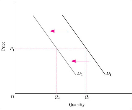
Figure 4 shows such a shift in demand. This figure does not have a numerical scale on the axes, as in Figure 3. Instead, the axes are just labelled ‘Price’ (P) and ‘Quantity’ (Q). ‘Quantity’ should be understood as ‘quantity per period of time’, such as a day, a week or a year. Diagrams such as this allow us to focus on the direction of change of variables and their implications, rather than exact magnitudes. Let us suppose that consumer incomes fall, so that everyone has less to spend on normal goods. The quantity demanded will therefore decrease at all prices. For example, at price P1 quantity demanded falls from Q1 to Q2. This means that we now have a new relationship between quantity demanded and price, and this is shown by the new market demand curve D2 in Figure 4 lying to the left of the original one, D1.
The key points about movements along and shifts of the market demand curve are:
If the price of the good changes while all other variables remain the same, this is reflected in a movement along the market demand curve.
If a variable other than the price of the good itself changes, the whole curve shifts, showing that after the change in the variable more (or less) is now demanded at each price.
Here is an exercise to help you think about shifts in the market demand curve.
Exercise 1
Think for a few minutes about how other things besides price may not remain equal in the market for electronic personal organisers. Work out what effect each will have on the demand curve. Then see if you can complete Table 1 below.
| Change in variable | Effect on demand curve |
|---|---|
| Decrease in income | Decrease in quantity demanded at all prices. Demand curve shifts to the left |
| Increase in income | |
| Rise in price of a substitute | |
| Fall in price of a substitute | |
| Rise in price of a complementary good | |
| Fall in price of a complementary good | |
| Change in socio-economic influences in favour of electronic personal organisers | |
| Change in socio-economic influences away from electronic personal organisers |
Discussion
| Change in variable | Effect on demand curve |
|---|---|
| Decrease in income | Decrease in quantity demanded at all prices |
| Demand curve shifts to the left | |
| Increase in income | Increase in quantity demanded at all prices |
| Demand curve shifts to the right | |
| Rise in price of a substitute | Demand curve shifts to the right |
| Fall in price of a substitute | Demand curve shifts to the left |
| Rise in price of a complementary good | Demand curve shifts to the left |
| Fall in price of a complementary good | Demand curve shifts to the right |
| Change in socio-economic influences in favour of electronic personal organisers | Demand curve shifts to the right |
| Change in socio-economic influences away from electronic personal organisers | Demand curve shifts to the left |
3 Firms, costs and technology
3.1 Introduction
In this section the focus turns towards the supply side of the market, towards firms and industries, exploring the importance of costs and technological change in the organisation of production. The objective is to understand some of the different kinds of change in industrial structure, namely changes in the number and size of firms in an industry. One such change saw the emergence of Ford, initially one among many similar firms jostling for position in the US automobile industry, as the industry ‘leader’. What was so special about Ford? Henry Ford was the first car maker to introduce an innovative assembly-line production technology. This gave him a competitive advantage over firms using more traditional and, for that reason, more expensive processes. Since consumers were unwilling to pay higher prices for broadly similar products, Ford's rivals were forced to take up the same new methods of production if they wanted to compete.
This story raises some important questions about competition, technology and costs. How do firms respond to changing conditions in their industry? What can a ‘typical’ firm do to cut its costs? What are the main constraints on its behaviour? Economists use models of the relationships between technology, costs and output of firms to explore these questions. This section examines these relationships in a basic economic model of a firm. It explores the scope the firm has for cutting its costs in the short and long run, and the impact of changing technology on the firm's costs. The distinction between the short run and the long run is important because it is based on assumptions about how much room to manoeuvre the firm has in responding to changing market conditions and draws attention to the role of investment in the firm's response. It is in the short run that the firm's actions are subject to the greatest constraint. In the analysis in this section, firms take technology as given. In Section 4 we remove this constraint, restoring to firms some influence in shaping technology and hence their costs to their own advantage.
3.2 Technology and costs in the short run
Advertising leaflets are dropping through letter boxes around the UK, as we are writing this chapter, from cable suppliers trying to attract new customers for their services. They promise to provide a telephone line, a bundle of television channels, an Internet connection, home shopping and movies-on-demand, all at a ‘bargain price’. These leaflets raise some interesting questions. How does expanding output of cable services by selling to new customers make it possible to offer them for sale at a lower price? What happens to the costs of producing cable services as the firm increases its output of them?
In analysing the costs, technology and output of firms, economists create a model of the typical or representative firm. A firm is an organisation that buys inputs, such as land, labour and capital, and transforms them into an output of goods and services for sale. We call these inputs to the firm's production process factors of production.
A firm that wants to expand output is likely to need more inputs. For example, in order to increase output the cable supplier would probably recruit more workers, such as the technicians who install cable boxes in customers’ homes and the telephonists who respond to customer enquiries. It might also need to buy in more of the equipment used by these workers, such as telephones, computers and engineering tools, and it might need to rent more office space. In other words, the firm increases its input of factors of production, namely labour (the technicians and telephonists), capital (telephones, computers and engineering tools) and land (office space). The firm is assumed to have done this by purchasing the additional inputs it needs from the relevant factor markets, for example by recruiting new workers in the labour market.
The firm can combine factors of production in various ways to create output, but is limited by the technology available to it. The best production methods available to the firm are summarised in its production function, which identifies the maximum output a firm can produce from each available combination of inputs. We can write it out using algebra in exactly the same way as we wrote out the demand function in Section 2:
This says that the firm's output (Q) (the dependent variable) is a function of the various factors of production (the different Fs, up to any number ‘n’ of them) such as land, different types of labour and machinery (the independent variables). This production function is the firm's technology. The firm is assumed to do the best it can with its inputs, without waste. If there is technological change, the firm can get more output from its inputs, that is, increase their productivity. In the models we discuss in this section all firms have access to the same technology.
The firm's objective is not to produce maximum output, but rather to make as much profit as possible. However, reducing costs is an important competitive tool in the search for profits, as the cable supplier's offer of a ‘bargain price’ to new customers illustrates. So how do firms’ costs change as output changes? What makes it possible to supply more customers at a lower price? Are there any limitations to this process? The distinction between the short run and the long run helps to answer these questions.
Question
We referred above to the cable supplier recruiting new workers. Can you think of any employers or industries that have found this difficult?
Discussion
In 2001 in the UK the health and education industries were beset with staff shortages and in some areas recruited from overseas. It is likely to take most employers longer to increase the quantity of skilled than unskilled labour. Skills may not be available in the locality and workers may have to be enticed to move from other jobs, involving periods of notice. New workers may have to be trained and the training period may well be lengthy. BBC television reported on 4 September 2001 that Arriva, a UK train and bus operator, had announced the cancellation of up to a hundred services a day because of a shortage of train drivers. Arriva had the capital equipment, the trains, to run the services but could not do so until it had increased the amount of skilled labour at its disposal by training new drivers. In this example the firm is constrained in its response to the demand for rail services because the quantity of one factor of production, labour, is fixed.
Economists describe the situation in which Arriva finds itself as the short run. A firm is operating in the short run when it is unable to change the quantity it uses of at least one of its factors of production. In other words, in the short run the firm can vary the quantity it uses of some of its factors of production but there is at least one which is fixed. The term denotes this constraint on the firm's behaviour rather than a particular period of historical time. The firm's actions take place in actual or historical time and so the short run will eventually come to an end, in Arriva's case when the drivers have been trained in a matter of months. Therefore, the short run, understood as the condition of being unable to change the quantity used of at least one factor, refers to different periods of historical time, depending on the circumstances of each particular firm. Another example from transport illustrates this variety. London's Heathrow, Stansted and Gatwick airports are constrained in responding to rising demand for air travel from London and south-east England by the planning process required before new runways or terminals can be constructed. In this case the fixed factor is capital and the short run is measured in years, perhaps even decades.
Heathrow Terminal 5 to get go-ahead
After an inquiry that began in 1995, the government is poised to give the go-ahead for Heathrow's Terminal 5. It is due to open in 2007, subject to final approval.
(Adapted from The Sunday Times, 4 November 2001, p. 2)
In the short run, therefore, the firm has one or more variable factors of production but at least one fixed factor. How does the firm's output change in the short run as it increases the amount of a variable factor? For example, let us suppose that the cable supplier recruited more labour, such as technicians and telephonists, while using unchanged quantities of both capital and land. Hiring more labour allows it to increase output. Initially, output may rise faster than the inputs of labour. Each additional worker may not need a computer all to themselves and, up to a point, extra workers can share the same office space. So initially increases in the amount of labour may generate larger ‘returns’ in the form of increases in output. At this stage in its expansion of output in the short run, therefore, the firm is experiencing increasing returns to a factor of production, in this case labour.
However, this fortunate situation has its limits. If the firm continues to expand output by increasing the input of labour with unchanged inputs of capital and land, a point will be reached after which the employment of even more workers brings successively smaller increases in output. For example, there may be so many workers that each one spends some time idle in the queue waiting to use a computer. The input of labour is rising faster than output, and the firm is now experiencing diminishing returns to a factor of production. Diminishing returns pose a serious constraint on the expansion of a firm in the short run.
These relationships between inputs and outputs in the short run influence the firm's costs. Returning to the cable supplier, it is now possible to frame a more precise question: what happens to the costs of producing these services as the firm increases its output of them in the short run? To analyse this, we need to distinguish total costs (TC) and the average cost (AC) of production. A firm's total costs are the expenses incurred in buying the inputs necessary to produce the firm's output. Average cost is the cost per unit of output. Average cost (AC) is therefore the total cost of production (TC) divided by the number of units produced (Q):

We can draw a short-run average cost (SRAC) curve that models the relationship between different levels of output and average cost (AC) in the short run (Figure 5). Each point on the SRAC curve represents the average cost in the short run (measured on the vertical axis) of producing a quantity of output (measured on the horizontal axis). Output (Q) is measured per time period, such as a year. The SRAC curve is expected to be ‘U’-shaped, as shown in Figure 5. The downward-sloping section of the SRAC curve indicates that as output expands from a low level, average costs in the short run fall. Eventually, however, the SRAC curve begins to slope upwards, showing that at output levels above Q1average costs rise as output increases.
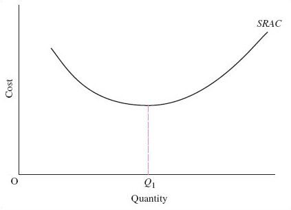
The shape of the SRAC curve arises from the technical constraints on short-run output expansion just described. We assume that the price of inputs is constant. As output expands the fixed cost of the fixed factors of production, such as the cable system itself, is being spread over an expanded number of customers. Increasing returns to a factor of production means that output rises faster than the variable input, so the cost of the variable factor per unit of output falls too. So initially the average cost of production (AC) falls as output rises.
Eventually, however, diminishing returns to the variable factor of production sets in. Output starts to rise more slowly than the variable input so the additional cost required to produce additional units of output starts to rise. Eventually total cost (fixed plus variable costs) will start to rise faster than output: that is, average costs will start to rise. On Figure 5 this happens as output rises above Q1.
To sum up, in the short run the firm's ability to reduce costs as output rises is constrained by diminishing returns. In the long run, opportunities to invest in factors such as plant and machinery mean that the quantity of all factors of production can be varied. How does that affect the firm's costs?
3.3 Long-run costs and economies of scale
What makes it possible to offer more output for sale at a lower price? That was one of the questions with which Section 3.2 opened. Part of the answer is that the firm's cost curves, which reflect the technology it is using, may display falling average cost as output increases over a range of output levels. The other part of the answer is that market demand must be sufficient to justify successive expansions of output. A firm such as the cable supplier seeking to increase sales by offering ‘bargain prices’ to its new customers is making an assumption about the size of the market. This section examines the relation between output and average cost on the assumption that the size of the firm's market is sufficiently large to justify increases in its input of all factors of production.
There is greater scope for cutting costs in the long run. In the long run the firm can increase inputs of all factors of production: labour, capital and land. This corresponds in reality to firms making investments. Firms invest in labour by training key personnel such as train drivers, technicians and telephonists. They may invest in items of capital equipment from telephones and computers to new factories or warehouses. They may invest in land by buying more office space or, literally, perhaps by buying a ‘greenfield’ site for a new runway. In modelling firms in the long run, it is still assumed that they are operating with given technology available to all firms.
How exactly do economists analyse the effects of investment of this kind on the firm's costs? The long-run average cost (LRAC) curve models the relationship between changes in output and average cost (AC) in the long run (Figure 6). Each point on the LRAC curve represents the average cost, in the long run, of producing a given quantity of output. The shape of the LRAC curve varies with the technology in use by firms in a particular industry. An increase in output in the long run is described as an increase in the scale of production, the phrase reflecting the implications of investment in plant and equipment. In the long run, a firm can adjust the quantities of all its factors of production to produce its desired level of output at the lowest possible cost. To achieve higher levels of output, a firm will need to buy more factors of production. How will costs change?
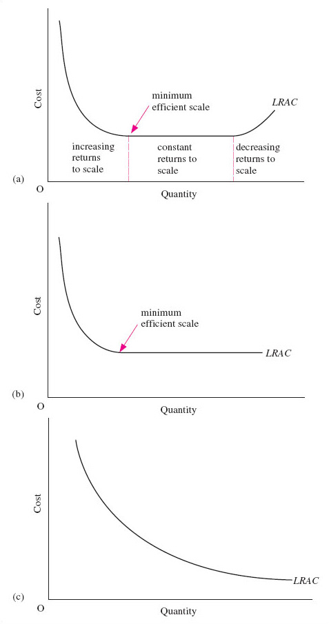
Figure 6 shows three possible shapes for the firm's long-run average cost (LRAC) curve. All three have a downward-sloping section: in (a) and (b) this occurs at low output levels; in (c) LRAC slopes down continuously over the whole output range. If the LRAC slopes downwards, the firm is benefiting from increasing returns to scale or economies of scale over the relevant range of output. We will use these two terms interchangeably. They both refer to a decrease in long-run average costs as output increases.
Increasing returns to scale arise within the firm from the firm's production function. Increased output may allow a firm to use inputs more productively. If doubling all the firm's inputs more than doubles output, there are increasing returns to scale. This may be because there are economies of increased dimensions. For example, enormous oil tankers and very large lorries can transport goods at lower cost per unit than smaller ships and vehicles because their capacity rises faster than the materials needed to make and run them. Industrial plant displays the same effect: building a factory extension that doubles the output capacity of the firm may be possible without doubling the costs of using and maintaining it. Furthermore, larger scale may also allow the more efficient use of inputs through specialisation of tasks.
The firm may also benefit from economies of scale that arise from sources outside the firm. These are reductions in a firm's average costs arising from the expansion of the industry to which it belongs. For example, the first IT firms which located in what has become known as Silicon Valley in the USA – or in Silicon Fen as the area around Cambridge, UK, is sometimes called – gained economies of scale when the industry began to expand. The concentration of numerous, closely related high-tech companies in a single geographical area meant that highly specialised factors of production (e.g. computer technicians and silicon chips) were available to them more cheaply and easily than they were to firms located elsewhere.
Firms may find that there is a limit to the economies of scale that they can achieve, a situation shown in Figure 6 (a). They will reach a level of output after which no further reductions in average cost can be obtained. This level of output is known as the minimum efficient scale (MES). The MES marks the size of the firm beyond which there are no cost advantages to be reaped from operating at a larger scale, or the output at which long-run average costs first reach their minimum level as output rises. In other words, it is the point at which all economies of scale have been taken up. As Henry Ford's smaller rivals discovered, once large-scale assembly-line production had been developed serious cost disadvantages were incurred by a firm operating below the MES, where average cost is higher than it would be if all scale economies were to be exploited. The MES is located at the beginning of the flat section of the LRAC curve, over which average cost is constant in Figure 6 (a). The firm is experiencing constant returns to scale over this range of output. Constant returns to scale exist when long-run average cost remains unchanged as output increases.
The LRAC curve depicted in Figure 6 (a) rises at high levels of output. Average costs increase as output increases. The firm is now experiencing decreasing returns to scale or diseconomies of scale. Decreasing returns to scale or diseconomies of scale exist when long-run average cost rises as output increases and arise from the disadvantages that large-scale production may entail. The major source of diseconomies of scale is the co-ordination problems that beset management in large bureaucratic organisations. The rapid expansion of an industry may also cause external diseconomies of scale, if labour costs increase as more and more firms chase scarce supplies of specific skills. For example, firms in some ‘new economy’ industries find wages are being bid up because of a shortage of workers with the appropriate IT skills.
The ‘U’-shaped LRAC curve shown in Figure 6 (a) is only one of three possible shapes that are usually distinguished. If the technology of the industry in which the firm is active is different from that of another industry, this will be expressed in a different LRAC curve. In Figure 6 (b) the LRAC curve is ‘L’-shaped, indicating that the firm continues to experience constant returns to scale across its output range once output is above the MES. This might correspond to a firm that can continue to replicate its production processes, for example by adding additional assembly lines, each one exactly like the others.
A third possibility is depicted in Figure 6 (c), where the firm enjoys economies of scale right across its output range. There is, therefore, every incentive, in the form of ever lower average costs, for firms to continue to expand output. A single firm can supply the whole market at a lower cost than could be achieved by a number of firms in competition with each other. Network industries such as gas, water and electricity distribution, fuel retailing, railway track and cable networks in telecommunications are examples of industries where firms are appropriately modelled by the LRAC curve shown in Figure 6 (c).
The three LRAC curves in Figure 6, considered together, imply that the technology of an industry is expressed in the shape of the particular LRAC curve used in modelling that industry. There is a further implication, which is that technology, reflected in costs, shapes the structure of the industry. If, for the moment, the ‘structure’ of an industry is understood to mean the number and size of firms that are active in it, this point can be illustrated in a number of ways. You have already seen that the US automobile and PC industries experienced a ‘shake-out’ of small firms as product standardisation enabled the exploitation of economies of scale.
In industries in which firms experience constant returns to scale there will be a minimum level of output, the MES, at which constant returns set in, that firms must be able to sustain if they are to remain competitive. The MES varies with the particular technologies characteristic of different industries. For many parts of the clothing, footwear and furniture industries, all economies of scale may be exploited at relatively low levels of output and so the MES is low relative to market size. By contrast, in industries such as automobiles and chemicals where economies of scale are available over much greater ranges of output, the MES is much higher in relation to the size of the market.
Question
What does this suggest to you about the number and size of firms in the clothing, footwear and furniture industries compared with those in automobiles and chemicals?
Discussion
There are likely to be fewer but larger firms in the automobile and chemical industries compared with the clothing, footwear and furniture industries. In the former, the exploitation of economies of scale up to high output levels relative to market size leaves room for only a few large firms in the market. In the latter, increasing returns to scale are exhausted at lower output levels relative to market size so there is room for more firms. In automobiles and chemicals the model predicts greater pressure for mergers and acquisitions as firms seek to expand output by taking over rival firms.
The existence in some industries of a level of output beyond which decreasing returns are experienced sets a limit to the size of firms and hence to the pressure for mergers and acquisitions. In fact, decreasing returns to scale can lead to the break-up of very large firms so that management can focus on making the ‘core’ business more competitive. The break-up of the chemicals firm ICI into ICI and Zeneca in 1993 can be interpreted as an example of this kind of behaviour.
If increasing returns are available across the whole output range required to supply the market, this has dramatic implications for industry structure. A single producer can supply the entire market at a lower cost than two or more competing firms. This is because a single firm avoids the cost of duplicating distribution networks such as gas, water and electricity pipes, railway track and telecommunications cables.
The technology of an industry, expressed in the shape of the LRAC curve of its firms, is therefore a major influence on the structure of that industry. However, in modelling firms’ costs in the short run and the long run, it has been assumed that firms are operating with given technology. It is now appropriate to relax this assumption and investigate the role of technological change in shaping industrial structure.
As Section 3.2 explained, a firm's production function embodies its technology. The model assumes that technology is given and is available to all firms in an industry. We can therefore think of technological change as a change in each firm's production function. Particular input combinations now become more productive, producing more output. What effect does this have on the long-run average cost curve?
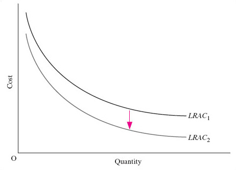
The LRAC curves in Figure 6 were drawn on the assumption of given technology. Technological change can therefore be understood as a shift in the average cost curve. Figure 7 shows a downward shift in an LRAC curve like that shown in Figure 6 (c). The shift of LRAC1 downward to LRAC2 in Figure 7 shows that long-run average costs have fallen at each and every level of output, or scale of production.
Technological change may not affect average costs at all levels of output. Henry Ford's introduction of moving assembly-line production methods is an example of a technological change that changed the shape of the LRAC curve for firms in the industry, shifting it downwards at high levels of output. The new methods hugely extended the range of output over which firms could benefit from increasing returns to scale. In this way, technological change, and its associated cost changes, exert a major influence on industrial structure. We explore this further in Section 4.
Exercise 2
A revision exercise before you move on.
Explain the meanings of the concepts listed below and how the items in each pair of concepts are related:
(a) increasing and diminishing returns to a factor of production;
(b) economies of scale and increasing returns to scale;
(c) decreasing returns to scale and diseconomies of scale.
Why do short-run average costs differ from long-run average costs?
Discussion
-
(a) Increasing returns to a factor of production occur when output increases faster than the input of a variable factor; decreasing returns to a factor of production refers to the opposite situation, in which output increases more slowly than the input of a variable factor.
(b) Economies of scale and increasing returns to scale are used interchangeably; both refer to a decrease in long-run average costs as output increases.
(c) Decreasing returns to scale and diseconomies of scale are used interchangeably; both refer to an increase in long-run average costs as output increases.
Short-run average costs differ from long-run average costs because in the short run at least one factor of production is fixed in quantity, resulting in diminishing returns to each variable factor of production above some level of output.
4 Technological change and industrial structure
4.1 Introduction
This section will explore the interaction of technology and costs with market demand in shaping industrial structure throughout the industry life cycle. Many industries begin as a numerous and turbulent group of firms jostling for position, experimenting with new and idiosyncratic products, and turn into a much smaller, more stable number of firms, making standardised products by routine methods. In this section we add a rather different view of firms to that developed in Section 3, modelling firms as dynamic agents engaged in a learning process and an active search for technological innovation. The term ‘dynamic’ signifies that the model constructs firms and industries as acting and undergoing change in historical time. The technology available to firms is no longer being assumed to be given from outside the firm. The industry life cycle, outlined in Section 4.2, provides a theoretical framework for identifying general patterns of structural change across different industries. Section Section 4.3 discusses some additional concepts used in modelling the dynamics of industrial structure.
4.2 The industry life cycle
The model of the industry life cycle represents an industry as if it were a biological organism going through the stages of birth, growth, maturity and decline. This helps us to understand how a particular firm can become the ‘leader of the pack’ through innovation. In Section 2 it was explained that an economic model is a deliberate simplification of the world, which helps to provide a systematic way of thinking about causal relationships. The industry life cycle is a rather different type of model. The aim is still to provide a systematic way of thinking about economic activity but not by analysing particular interactions between variables. The industry life cycle is instead a systematic way of thinking about general patterns of structural change across different industries. In this sense, the industry life cycle is an ‘ideal type’, enabling us to bring order to the complexity of historical events by classifying them as belonging to this or that phase of an identified pattern of industrial change.
The industry life cycle models industries as following a similar pattern of development as industry output changes, moving from many small and different firms to a few large and similar firms. This change in industrial structure is driven by the interplay between consumer demand and technology throughout the industry life cycle. Section 2 examined some of the influences on market demand and the particular importance of price. In fact, price and non-price factors are of varying importance at different phases of the life cycle. Section 3 analysed the firm's SRAC and LRAC curves, which reflect the technology available to the firm. Costs are of crucial importance to the firm at each phase of the industry life cycle but firms are driven to focus on costs in different ways at different phases.
The model of the industry life cycle is depicted in Figure 8. The curved line traces how the total output of a typical industry changes over time. In this diagram, the total output of the industry is measured along the vertical axis. The horizontal axis shows the passage of time.
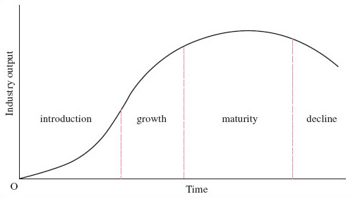
The introductory phase is characterised byproduct innovation, that is, the introduction of novel products for which there are no close substitutes. At this stage the scale of production is low, costs are high and demand for the new industry's products is limited to relatively few consumers. There will be considerable variety among firms in the industry, ranging from small firms that are as new as the industry to large firms with established products in other industries that are diversifying into the new one. Some firms will have entered the industry right at the start, while others enter more gradually as the profit opportunities created by the original ‘pioneers’ become clear. This ‘heterogeneity’ among firms, that is, their variety, will be reflected in differences in the technology they use and hence in the costs that they face. Hence technology is no longer understood as ‘given’ and common to all. The experimental nature of production at this stage favours firms that can learn quickly and are therefore able to be more flexible and better able to adjust output rapidly in response to changing conditions. In the introductory phase of the industry life cycle, production is a risky business and firms cannot be sure that their product is exactly what consumers want.
You can see, in Figure 8, that as the industry moves from the introductory phase into the growth phase, the size of the industry, measured in terms of its output, increases. Firms will be able to exploit economies of scale. There is, however, a condition. The selection of 35 mm SLR film cameras and digital cameras shown in Figure 9 holds a clue about the condition for achieving economies of scale.
4.2.1 Figure 9a: A selection of 35 mm SLR film cameras
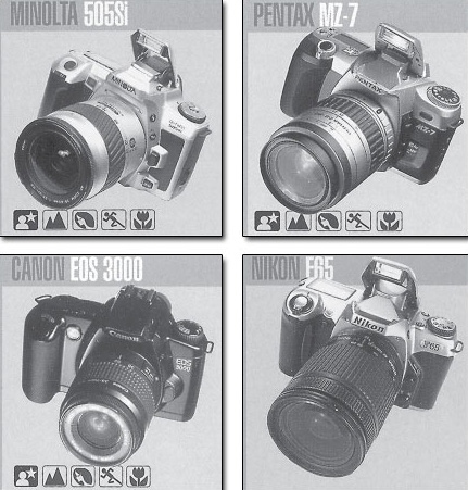
4.2.2 Figure 9b: A selection of 35 mm digital cameras

Question
What do you think is the main difference between the appearance of the 35 mm SLR film cameras and that of the digital cameras in Figure 9?
Discussion
There is considerable variety among the digital cameras. At first glance the Fuji Finepix 6800 resembles a hand-held computer; the Fuji Finepix 40i looks to us like a portable CD player and is in fact an MP3 player as well as a digital camera; and the Nikon Coolpix 950 is perhaps too radical a design to be mistaken for anything else. On the other hand, the Fuji Finepix 4900 looks much more like a 35 mm SLR film camera. This variety and sense of experiment is consistent with the digital camera industry being in its introductory phase. Manufacturers seem undecided whether a digital camera should look like a computer with a lens or a camera with some data-processing software. By contrast, it seems to us that the 35 mm SLR cameras are remarkably similar in appearance and they are also similar in technical specification. Standardisation is evidently lacking among digital cameras. Product standardisation is symptomatic of a move to the growth phase of the industry life cycle. Once firms have standardised the product, they can also standardise the manufacturing process and move to production on a large scale.
Question
What advantages will this move to production on a large scale confer on firms in the growth phase of the industry life cycle?
Discussion
The advantages of large-scale production, summed up in the concept of economies of scale, or increasing returns to scale (Section 3.3), generate a revolution in industrial structure once the expansion of demand gets under way. On the supply side, increasing returns to scale at the growth stage of the cycle can be exploited by the largest and most efficient firms as they compete and survive. Those firms that have failed to keep pace with changing opportunities exit from the industry; that is, a ‘shake-out’ takes place. This contraction in the number of firms means that the industry exhibits a greater degree of concentration as a few large firms dominate the industry. For example, from 1909 to the mid 1920s the number of firms in the US automobile industry fell from 271 to approximately 50 and the number of firms in the US PC industry showed an equally dramatic decline during the years from 1973 to 1999.
How might this be explained? On the demand side, the fall in average costs resulting from increasing returns makes it possible for the firm to reduce the price it charges for the new product. This sequence of events was encountered in the extract from The Economist's survey of the new economy at the beginning of Section 1. The suggestion was that new technologies are a major cause of the decline in costs and hence in prices that enables large numbers of consumers to buy safer cars, personal computers and so on. In terms of the model of market demand explained in Section 2, the fall in price leads to a movement along the market demand curve, bringing the product into the range of many more consumers. This is reinforced by a shift in the market demand curve caused by a change in socio-economic influences, in particular the demonstration effect that describes the tendency of people to imitate the consumption decisions of those who have already bought the product (Section 2.3).
The phase of maturity is reached as the market approaches saturation and replacement demand becomes important. By now there are many similar products for consumers to choose from, as they replace their first car or washing machine – or 35 mm SLR camera – and price exerts a major influence on demand. By the mature phase, the product has become well established and most of the consumers who would like one have already acquired it. The quantity demanded is therefore relatively stable and this is reflected in a flattening of the curve in Figure 8. Firms now have to work hard to reach those consumers who still have not bought the product and to create a demand for replacement purchases. The UK domestic appliance industry provides a good example of this phase. Most of the consumers wanting to own a refrigerator now have one and so the main source of market demand lies with consumers setting up home for the first time, and those needing to replace old equipment. Since there are plenty of very similar products available, price is a key determinant in deciding which one to buy.
On the supply side the focus of the firm's attention therefore shifts to process innovation aimed at securing reductions in the average cost of production. For example, Henry Ford found that the way to drive down costs is through the introduction of innovative new manufacturing processes. The firm that fails to innovate and to adopt industry best-practice technologies of production soon finds that it cannot compete with the lower prices offered by its rivals and is forced to exit the industry. In these circumstances the aim of investment may be to enable a firm to ‘catch up’ with its competitors by introducing the best available technology already in use elsewhere. A good example of this is provided by the German car manufacturer BMW when it took over the Longbridge car plant in the UK. BMW brought the factory up to date with the technologically advanced methods of car production introduced into the UK when the Japanese firms Nissan and Toyota set up new factories near Sunderland and Derby respectively.
Finally, the industry enters into decline when new industries with new products embodying superior technology render the old industry's products obsolete. This phase may be brought on by further product innovation giving rise to a new industry with its own introductory phase so that radically new products replace the obsolete ones. For example, the development of synthetic materials in the 1960s meant that a wide range of industries using ‘natural’ materials went into decline. Some of the firms in these industries, such as carpet manufacturers, were able to draw on the new materials to reinvent their products, but others disappeared altogether as demand for their products dissolved.
Each stage of the model of the industry life cycle presented above is fixed and distinct. In reality, the boundaries between stages in the development of an industry are blurred and can be difficult to observe in a short time horizon. The length of the life cycle also varies with the extent to which the products it makes can be reinvented. The personal stereo industry offers an example. By the 1980s, many consumers already owned a personal stereo that played audio-cassettes. With the arrival of new technologies for recording music on CDs, consumers shifted from cassettes to CDs in order to benefit from better recording quality. This stimulated a replacement demand for personal stereos that could play CDs, extending the life cycle of the personal stereo industry.
4.3 Industrial dynamics: knowledge and network industries
This final subsection introduces two more concepts that develop further our analysis of the dynamics of industrial structure, with particular reference to the ‘new economy’ industries. A dynamic approach to industrial change places considerable emphasis on innovation and learning, seeing firms as actively searching out innovative products and processes and learning how to produce and sell them. Some of the novelty of the new economy is reflected in the concepts used in trying to understand it, which are applied here to a brief analysis of network industries.
4.3.1 Knowledge and learning in the industry life cycle
In Section 3 we described technology as ‘given’ to firms. Now let us reflect on that idea. We can think of technology as consisting of bodies of knowledge necessary to produce artefacts. An appreciation of the importance of knowledge to economic activity is not new, for it was recognised by the eminent economist Alfred Marshall, who wrote that ‘Capital consists in a great part of knowledge and organisation’ (Marshall, 1925, p. 138). What Marshall meant can perhaps best be understood by considering two ‘thought experiments’ broadly similar to those conducted by the philosopher Sir Karl Popper. In the first, all human artefacts, and hence all capital equipment, are wiped out in an extraordinary natural disaster. Human beings survive unharmed and set about constructing their capital stock, and other artefacts, all over again. This is an immense task but in a decade or so the job is done. In the second thought experiment we imagine once again that all capital equipment is destroyed. The difference is that this time human knowledge is also lost. All memories of how to build lathes, computers, robots, cars, combine harvesters and all the other machines the human race has ever invented are annihilated and so too are all the skills acquired in learning how to use them. The human race effectively returns to a much earlier period in its evolution when the capital stock consisted perhaps of stone tools. Even supposing that history repeats itself and people eventually reinvent the technologies leading up to the capital stock of twenty-first century humanity, it would take thousands of years to get back to where we were. The hardware is important but it is human knowledge that really matters. Learning how to use the hardware most effectively is therefore a crucial capacity for firms.
The ‘learning curve’ captures the idea that turning technological change to competitive advantage is a skill that has to be learned like any other. Figure 10 depicts this idea. It shows a fall in average cost that occurs as learning takes place over time after the firm starts up in production. This figure looks rather like the LRAC curve in Figure 6 (c) but depicts a different relationship between output and costs. The horizontal axis, labeled ‘cumulative output’, shows the output a firm produces each year added together over time. This contrasts with the SRAC and LRAC diagrams in Section 3, where output was measured per time period, such as a year, and the diagrams picture the firm's costs at any given output per year. In Figure 6, a firm might move left or right, depending on its output decisions for the year. However, in Figure 10 you should think of the firm as moving rightwards over time, since each year it continues in business, cumulative output will necessarily increase.
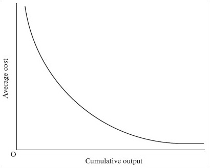
When a firm benefits from learning-by-doing, it is said to be ‘moving along the learning curve’ or gaining from ‘experience effects’. Learning-by-doing refers to a fall in unit costs as cumulative output increases. Imagine that the production process involves the use of a new machine. When a worker first starts to operate the machine, lack of familiarity means that mistakes are made and progress is slow. However, the worker learns from these mistakes and as the hours spent operating the machine increase, productivity improves, that is, more units of output are produced per unit of input. The more cumulative output is produced, the more efficiently it is produced. The cost of producing a unit of output therefore declines as cumulative output increases, as Figure 10 shows.
Learning effects are not confined to assembly-line tasks but can occur throughout the firm wherever repetition gives rise to experience. Their significance in the industry life cycle is greatest when firms are learning how to use new technology. This occurs both in the introductory phase, as firms experiment with new products, and in the mature phase, as firms learn how to use new processes to improve the manufacture of a standard product. As the point is reached when all the cost savings derived from experience have been extracted, there is a flattening of the learning curve (Figure 10). From then on the firm diverts its attention to other ways of reducing its costs as a means of gaining an advantage over rivals.
A firm's capacity for learning how to use new technology depends in part on whether innovations build on its existing strengths or render them obsolete. Many historical studies have documented how technological change (process or product innovation) does not evolve in a continuous and smooth manner but discontinuously. A long period of incremental change may be punctuated by episodes of radical change. These discontinuities that are introduced by technological innovation can be classified as either ‘competence enhancing’ or ‘competence destroying’ (Tushman and Anderson, 1986).
To understand this, we need to recognise that once we allow firms to learn and innovate individually, we have moved away from the model of the firm presented in Section 3. That section modelled a ‘representative’ firm among very similar firms. Once firms can learn, we move away from this approach, towards modelling firms as diverse organisations that develop distinct capabilities or competencies over time. Competence-enhancing innovations are innovations that develop new products, or improvements to existing products, which build on a firm's existing competence and strengthen its market position. This cumulative ‘success begets success’ dynamic causes the market structure to become more concentrated, stable and less friendly for new firms:
Existing firms within an industry are in the best position to initiate and exploit new possibilities opened up by a discontinuity if it builds on competencies they already possess … the rich are likely to get richer.
(Tushman and Anderson, 1986, p. 444)
Competence-destroying innovations have the opposite effect. They develop new products or changes in existing products which require completely new skills and knowledge to be developed. These innovations disrupt industry structure, rendering current capabilities obsolete. Existing firms, set in the old way of doing things, are often not quick or ready enough to adapt to this radical change, allowing new flexible firms (not always small) to enter, remaking industry structure – and perhaps starting a whole new life cycle. Innovation can therefore either stabilise or destabilise industrial structure.
4.3.2 Network externalities and increasing returns to scale
The reader should ask herself the following question: Would I subscribe to a telephone service knowing that nobody else subscribes to a telephone service?
The answer should be: Of course not! What use will anyone have from having a telephone when there is no one to talk to?
(Shy, 2001, p. 3)
The uncertainty surrounding production in the introductory phase, which places such importance on the ability of the firm to secure quick benefits from learning effects, is particularly acute in ‘network industries’, such as telecommunications, computers, video players, banking services, fuel retailing and many others. On the demand side, the example of a telephone service shows that the benefit (or ‘utility’) that people get from consuming such goods depends on the extent to which other people also use these goods. These goods are said to display network externalities because the value one consumer gets from, say, a telephone depends on factors external to their own consumption of it. The idea of externalities is widely used in economics. Network externalities (which can also be referred to as ‘network effects’) thus ‘arise when the attractiveness of a product to customers increases with the use of that product by others’ (Fisher and Rubinfeld, 2000, p. 13); in other words, when the value of one consumer joining a network depends on the number of other consumers joining the network. The more people who subscribe to the same standardised system, the more services and people the user can access, and so the greater the value of that system to each individual user. The implication is that firms that are in the introductory phase of a network industry life cycle face huge rewards from establishing an early lead for their product. Even if competing products have more useful features, the product with the largest network will be difficult to dislodge simply because the number of its subscribers make it the most attractive option for new subscribers.
On the supply side there is considerable scope for the firm with the largest network to achieve increasing returns to scale. The firm faces the cost of developing and maintaining a single network, and that cost can be spread over a large and rising quantity of output, reducing average cost (AC). The industry life cycle models the transition to the growth phase as depending in part on product standardisation (Section 4.2). A stronger version of standardisation is present in network industries. The cost advantages are particularly dramatic for a firm that can establish its own network, or a technical component essential to the functioning of a network, as the industry standard.
Network industries have in common a number of characteristics including complementarity, compatibility and standards (Shy, 2001, pp. 1–3). A network industry produces complements, such as trains and railway tracks, cameras and film, computers and software, CD players and CDs, and cars and fuel. These complementary products must be compatible with one another in the sense that trains are no use unless they fit the tracks, film is needed if you want to use a film camera and so on. In other words, complementary products must operate on the same standard. For example, in the nineteenth century it was impossible for regional railway companies in the UK to run rolling stock on each other's tracks until a national gauge or width was established. This gauge is an example of an industry standard. Without a standard gauge or film size or computer operating system, product standardisation cannot take place and economies of scale are unobtainable. Establishing an industry standard may involve a struggle between competing would-be standards. When video players were first introduced in the 1980s, two different recording formats appeared on the market, VHS and Betamax. It was some years before VHS was established as the industry standard.
Case study: BMW wants to make internal-combustion engines that run on hydrogen
One way that global warming might be reduced is by powering cars with something that does not release carbon dioxide when it is burned. That is part of the idea behind a ‘hydrogen economy’ – a future in which hydrogen, which can be produced from renewable sources, takes over from hydrocarbons as the world's principal fuel.
Several of the world's car makers – notably Ford, DaimlerChrysler and Honda – are studying fuel cells. These react hydrogen and oxygen together to produce electricity. Fuel cells certainly work but they are still some years from commercial viability in cars. There is, however, an alternative: burn the hydrogen in a conventional internal-combustion engine. And that is what BMW proposes to do.
Converting an engine to run on hydrogen is relatively simple. There are, however, two catches. The first is that fuel cells are a far more efficient way to use hydrogen than burning it in a conventional engine. The second is that, gram for gram, hydrogen contains significantly less energy than petrol. Performance will reflect that, unless those clever engineers at BMW can somehow overcome the difference. If they cannot, then BMW, whose prestige and independence rely largely on its engine-making ability, may be in trouble. Were fuel cells to become the standard, the firm's future could be bleak.
(Adapted from The Economist, 21 July 2001, p. 86)
Question
This case study describes the situation facing car manufacturers as they develop new technology for the ‘hydrogen economy’ of the future. How does BMW's decision to use hydrogen in an internal-combustion engine illustrate the uncertainties confronting firms in network industries in the introductory phase of the industry life cycle?
Discussion
The new network industry in this case is hydrogen fuel production and retailing. A means of propulsion, such as an internal-combustion engine or a fuel cell, and a fuel, such as petrol or hydrogen, are complementary goods. The means of propulsion and the fuel must be compatible, in the sense that a conventional internal-combustion engine is compatible with petrol and a fuel cell with hydrogen. The industry can progress to the next phase of the life cycle only if an industry standard can be agreed upon. There seems to be a consensus that hydrogen will become the standard fuel. Beyond that, however, there is uncertainty. Ford, DaimlerChrysler and Honda are investing in fuel cell technology in the belief that it will become the industry standard in the ‘hydrogen economy’, while BMW take the view that the internal-combustion engine will retain that position in the new circumstances. The industry dilemma highlights the role of technological change in shaping industrial structure. If BMW have ‘backed a loser’ and invested in a technology that fails to become the industry standard, they may, as the case study suggests, lose their independence. The number of firms in the industry will decrease if BMW's destiny is to fail, as part of the process by which technological change shapes a new industrial structure.
Network externalities on the demand side and increasing returns on the supply side may interact in what is colloquially termed a ‘double whammy’ to produce a dramatically different industrial structure as an industry moves into the growth phase. A firm that benefits from such a double whammy will secure monopoly power in its industry.
5 Conclusion
The idea of the double whammy brings together the two driving forces behind changes in industrial structure, with which this course opened and now closes. The use of a new technology causes a decline in the costs of production, which in turn encourages a rapid take-up by consumers of products embodying the new technology. This course has explored the factors affecting consumer demand. While the price of the product was found to be of crucial importance, socio-economic influences such as culture and identity were seen to have an important role to play, especially in the introductory phase of the industry life cycle. It is also possible to explain the foundations of consumer demand with an account of utility theory and its role in understanding individual choice and equilibrium.
On the supply side the firm's cost curves reflect the technology it uses to produce goods and services. An analysis of cost curves showed the constraints imposed by technology on the firm's development and how technological change creates new opportunities. Technology is ultimately a matter of knowledge and technological change can best be modelled in dynamic terms, as firms search creatively for new products and processes and learn how to make and employ them.
In the network industries, prominent in the new economy, the demand- and supply-side factors interact in particularly striking ways. Network externalities and industry standards combine to push the industry from a turbulent crowd of heterogeneous firms to a small number of similar firms. It is also possible to put together the analysis of demand, costs and technology into a study of firms’ decision-making and of the behaviour of firms in industries where one firm is big enough to wield monopoly power.
6 Questions for review and discussion
Question 1
Complete the following sentences by selecting the correct word or phrase from the list below to fill in the spaces:
| independent |
| dependent |
| positive |
| negative |
| Giffen |
| Veblen |
| slope downwards from left to right |
| slope upwards from left to right |
| are horizontal |
| are vertical |
| are indeterminate |
A market demand curve shows the relationship between quantity demanded (the ……… variable) and price (the ……… variable). According to the ‘law of demand’, this relationship will be a ……… one. Some luxury goods called ……… goods, and some very basic goods, called ……… goods, are exceptions to the ‘law of demand’, and their market demand curves ………
Answer
A market demand curve shows the relationship between quantity demanded (the dependent variable) and price (the independent variable). According to the ‘law of demand’, this relationship will be a negative one. Some luxury goods called Veblen goods, and some very basic goods, called Giffen goods, are exceptions to the ‘law of demand’, and their market demand curves slope upwards from left to right.
Question 2
Figure 11 shows a hypothetical demand curve for cartridge pens. Draw a shift in the curve leftwards or rightwards as appropriate to illustrate the likely effect of each of the following:
(a) An increase in the price of fibre-tipped pens
(b) An increase in the price of ink cartridges
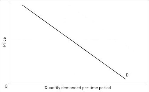
Answer
(a)
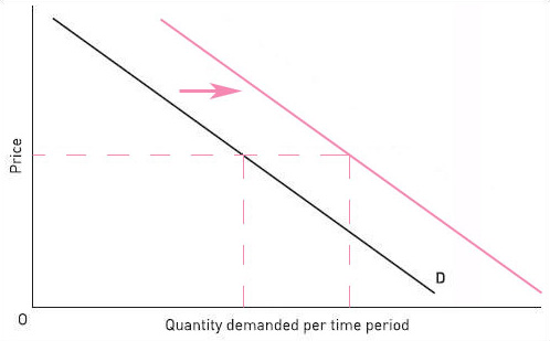
(b)
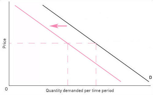
Question 3
Say which is the most appropriate phrase to complete the sentence below:
A firm is operating in the short run when…
(a) It cannot change the quantity it uses of any of the factors of production, so some inputs are being wasted.
(b) It is suffering diminishing returns to its fixed and variable factors.
(c) There is not sufficient time for it to raise its output.
(d) It cannot change the quantity it uses of at least one of its factor inputs.
Answer
(c) There is not sufficient time for it to raise its output.
Question 4
Figure 12 shows a short-run average cost curve for a firm. Select two statements from the list below. The statement you mark ‘1’ should state what happens as output rises from Q1 to Q2. The statement you mark ‘2’ should state what happens as output rises from Q2 to Q3.
Note: ‘average’ means ‘per unit of output’.
(a) Average fixed cost falls, average variable cost falls then rises.
(b) Falling average variable cost outweighs rising average fixed cost.
(c) There are diminishing returns to the variable factors throughout.
(d) Average fixed cost and average variable cost both rise.
(e) There are increasing returns to the variable factors throughout.
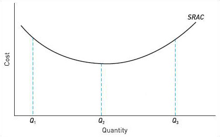
Answer
(a) Average fixed cost falls, average variable cost falls then rises.
(c) There are diminishing returns to the variable factors throughout.
Question 5
Figure 13 shows long-run average cost curves for two firms, A and B, each in a different industry. Select from the list of statements below the one that is consistent with what is shown in the diagram.
(a) Firm A attains minimum efficient scale (MES) at a lower level of output than Firm B.
(b) Both firms experience diseconomies of scale at the highest levels of output shown.
(c) Firm A operates in an industry where there is great pressure to expand output, for example by merger.
(d) Firm B has higher fixed costs than Firm A.
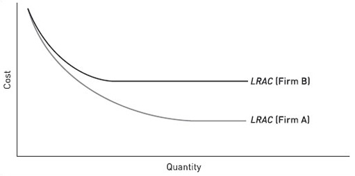
Answer
(c) Firm A operates in an industry where there is great pressure to expand output, for example by merger.
Question 6
Figure 14 shows a learning curve for a firm. The curve is similar in shape to a long-run average cost (LRAC) curve, but the relationship it depicts is different. Select from the list below the three statements that correctly identify differences between curves of these two kinds:
(a) The horizontal axis of the learning curve shows cumulative output; that of the LRAC curve shows output per time period.
(b) The costs shown by the learning curve exclude capital costs; those shown by the LRAC curve include capital costs.
(c) The firm moves rightwards along its learning curve over time; the firm may move leftwards or rightwards along its LRAC curve.
(d) At some points on the learning curve, factor inputs are being wasted owing to mistakes and inexperience; at all points on the LRAC curve, the firm uses all inputs to their full potential and there is no waste.
Answer
(a) The horizontal axis of the learning curve shows cumulative output; that of the LRAC curve shows output per time period.
(c) The firm moves rightwards along its learning curve over time; the firm may move leftwards or rightwards along its LRAC curve.
(d) At some points on the learning curve, factor inputs are being wasted owing to mistakes and inexperience; at all points on the LRAC curve, the firm uses all inputs to their full potential and there is no waste.
Question 7
Complete the following sentences by selecting words or phrases from the list below.
| representative |
| competence-enhancing |
| mature |
| distinct competencies |
| competence-destroying |
| manufacturing |
| network |
| reproduce competencies |
In analysing the costs, technology and output of firms, we can use a model of a ……… firm. But when thinking about innovation, we need to model firms as diverse organisations that develop ………
……… innovations tend to cause market structure to become more concentrated. The need to secure quick benefits from learning effects is particularly acute in ……… industries.
Answer
In analysing the costs, technology and output of firms, we can use a model of a representative firm. But when thinking about innovation, we need to model firms as diverse organisations that develop distinct competencies.
Conpetence-enhancing innovations tend to cause market structure to become more concentrated. The need to secure quick benefits from learning effects is particularly acute in network industries.
Question 8
The table below gives information about a firm's costs in the short and long run.
| Output (000s) | ||||||||||||||
|---|---|---|---|---|---|---|---|---|---|---|---|---|---|---|
| 1 | 2 | 3 | 4 | 5 | 6 | |||||||||
| Short-run average cost (£) | 18 | 9 | 9 | 11 | 14 | 14 | ||||||||
| Long-run average cost (£) | 18 | 6 | 5 | 5 | 5 | 6 | ||||||||
(a) Draw a diagram showing each of the above curves and explain briefly what distinguishes the short run from the long run.
(b) With reference to the diagram, explain how (i) diminishing returns and (ii) diseconomies of scale affect the production costs of a firm.
(c) With reference to the diagram, give an example of a change which can cause (i) a movement along the long-run curve and (ii) a shift of the long-run curve.
Question 9
Essay: Using examples, explain how network externalities and economies of scale interact to determine industrial structure.
References
Acknowledgements
The material below is contained in chapter 3 of Economics and Economic Change Microeconomics (2006) (eds) Graham Dawson, Maureen Mackintosh and Paul Anand, which is published by Pearson Education Limited in association with The Open University. Copyright © The Open University.
The material acknowledged below is Proprietary, used under licence and not subject to Creative Commons Licence (see terms and conditions). This content is made available under a Creative Commons Attribution-NonCommercial-ShareAlike 4.0 Licence
Grateful acknowledgement is made to the following source:
Extract in Section 4.3: ‘BMW wants to make internal-combustion engines that run on hydrogen’, The Economist, 21 July 2001. Copyright © The Economist Newspaper Limited, London.
Course image: Jerry Meaden in Flickr made available under Creative Commons Attribution-NonCommercial-ShareAlike 2.0 Licence.
Figure 1: Copyright © Citroën UK Ltd; Figure 2: Copyright © IPC Media Ltd; Figure 9: Copyright © IPC Media Ltd.
Adapted from Ole Wiemeler: [Details correct as of 15th February 2008]
Don't miss out:
If reading this text has inspired you to learn more, you may be interested in joining the millions of people who discover our free learning resources and qualifications by visiting The Open University - www.open.edu/ openlearn/ free-courses