Digital communications
Use 'Print preview' to check the number of pages and printer settings.
Print functionality varies between browsers.
Printable page generated Thursday, 25 April 2024, 6:50 PM
Digital communications
Introduction
This unit is from our archive and it is an adapted extract from Digital Communications (T305) which is no longer in presentation. If you wish to study formally at The Open University, you may wish to explore the courses we offer in this curriculum area.
By using optical fibre, very high data rates (gigabits per second and higher) can be transmitted over long distances (tens of kilometres) without amplifiers or regenerators. Optical fibre has completely superseded copper wires as the primary medium for cabled transmission over long distances. As demand for capacity has risen, fibre is now being used even in LANs and the access network. An understanding of optical-fibre communications is therefore very important for anyone with an interest in digital communications.
This OpenLearn course provides a sample of level 3 study in Computing & IT
Learning outcomes
After studying this course, you should be able to:
convert between wavelengths and frequencies
describe the main differences between lasers and LEDs as used as light sources for optical-fibre communications systems
describe the difference between direct and external modulation of a laser
describe the difference in structure and performance of step-index multimode, graded-index multimode and single-mode optical fibres
draw up a power budget for an optical-fibre communication link and use it to estimate the maximum link distance.
1 Optical fibre communication: introduction
1.1 Uses of optical fibre in communication
Using optical fibres, very high data rates (gigabits per second and higher) can be transmitted over long distances (tens of kilometres) without amplifiers or regenerators. As a consequence, optical fibre has completely superseded copper wires as the primary medium for cabled transmission over long distances. Until recently, however, optical fibre has been used less in LANs, where twisted-pair copper cable has been dominant. Similarly, fibre has been slow to penetrate the access network, from homes or businesses to the first telephone exchange.
Here I will make the distinction between the access network (from homes or businesses to the first telephone exchange – also called the last mile, local loop, or subscriber network) and the core network (between exchanges, also called the trunk network).
As demand for capacity has risen, however, the merits of optical fibre become ever more significant, and fibre is now being used even in LANs and the access network.
The way in which fibre is used is also changing. Originally, fibre was used just for stand-alone point-to-point links. Signal processing – amplification, regeneration, switching and routeing, for example – was done in electronic components. Now, however, devices for optical signal processing have been developed so that ‘all-optical networking’ is possible.
In this unit the basics of communication over optical fibre are covered in Section 2 and the components such as amplifiers and switches are introduced in Section 3.
1.2 Wavelength or frequency?
In this unit you will find frequent references both to the wavelength of light and the frequency of light. It is important to be able to work with both, and convert from one to the other. In the context of optical-fibre communication, the light radiation we are concerned with is usually in the infrared region of the spectrum.
To identify the position in the electromagnetic spectrum it is usual to refer to the wavelength of light, rather than its frequency. Thus I will refer to the ‘1300 nm window’ rather than the 2.3 × 10¹⁴ Hz (230 THz) window. T is the SI prefix ‘tera’, the multiplier for 1012.
When talking about the details of the optical spectrum both wavelengths and frequencies are used. In dense wavelength division multiplexing, for example, the carriers are often referred to by their frequencies rather than their wavelengths, and it is important to be able to convert readily from one to the other.
The conversion between wavelength (lambda, λ) and frequency (f) uses the formula:

where c is the speed of light in free space (i.e. in a vacuum) which is
3.00 × 10⁸ m s−1 to three significant figures. This may be rearranged to give:
Note that because the speed used is that of light in free space, references to wavelength are to the wavelength of the light in free space, which is different from (i.e. longer than) the wavelength of the same light in a fibre. When light enters a fibre from free space (or air) it slows down but the frequency remains the same, so the wavelength decreases.
You need to be careful when converting between wavelength and frequency spacings or ranges, rather than individual values. For example, let's suppose you know the output from a light-emitting diode (LED) contains wavelengths between 1300 nm and 1320 nm so that the spectral width is 20 nm and you want to know the frequency range in hertz.
To get the exact frequency range you need to convert each end of the range to frequencies and subtract one from the other. Thus the spectrum of the LED output in this example extends from
to
The spectral range expressed in frequencies is therefore:
Notice that you have to be careful with the accuracy of the intermediate steps in this calculation because it involves subtracting two large and similar numbers.
For small spectral widths there is an approximation formula to convert between spectral width measured in wavelength (Δλ) and spectral width measured in frequency (Δf):
where λ and f are taken at the mid-point of the range. This approximation is valid provided the fractions are small – less than about 1/10, for which we require Δλ
Often we may know λ but not f, so we can use f = c/λ to get:

and therefore:
Using the example of the LED again, taking λ in the middle of the range at 1310 nm gives:
SAQ 1
Suppose an LED has a spectrum that extends from 1540 nm to 1560 nm. Calculate:
its spectral width in nm
its centre frequency in Hz
its spectral width in Hz.
Answer
Its spectral width in nanometres is 1560 – 1540=20 nm.
Its central wavelength is 1550 nm, which corresponds to a frequency of
Its spectrum extends from
to
which is a spectral width of

Alternatively, this can be calculated using the approximation formula:
Notice that the spectral width of the LED in this SAQ measured in terms of wavelength was the same as that in the example given in Section 1.2, i.e. 20 nm. The spectral width measured in frequency is different, however: 3.5 × 10¹² in one case and 2.5 × 10¹² here. They are different because the centre wavelength is different.
2 Elements of an optical-fibre link
2.1 Light sources and detectors
The basic building blocks of an optical-fibre link are the light source, the fibre and the detector (Figure 1).
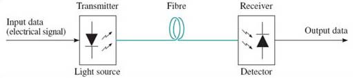
There are broadly speaking two categories of device used as light sources: light-emitting diodes (LEDs) and laser diodes. In general terms, LEDs are cheaper and easier to use, but have inferior performance compared to laser diodes.
The output from an LED differs from that of a laser diode as it is possible to couple more light power from a laser diode than from an LED to an optical fibre, and the spectral linewidth of an LED is much broader than that of a laser diode.
The lower power coupling from an LED comes partly from the fact that LEDs generally emit lower light power than laser diodes (the output from an LED is typically no more than −10 dBm), but also because the light from an LED spreads into a broader beam than the light from a laser diode. This latter point – the broader beam – means in particular that it is not possible to couple light from an LED very efficiently into a single-mode fibre, and in practice LEDs are only used with multimode fibre.
Single-mode laser diodes, can have spectral widths of 10 MHz or less. Narrow spectral width is particularly important at high signalling rates and in dense wavelength division multiplexed (DWDM) systems, so single-mode laser diodes are used in these systems. But there are further considerations that come into play to ensure a narrow spectrum – in particular, the mechanism used to modulate the light is important.
'Single-mode’, as used in ‘single-mode laser diode’, refers to a characteristic of the way in which the laser operates and of the resulting output spectrum. It does not have the same meaning as ‘single-mode’ as used in ‘single-mode fibre’.
The original – and cheapest – way to modulate a laser (or an LED) is to vary the electrical supply to the device. Modulation of an LED by a digital signal is done by switching the electrical current supplying the device on and off. Laser diodes can be modulated in a similar way, but for operation at high rates it is better not to switch the laser off completely so that the modulation is strictly ASK (amplitude shift keying) rather than OOK (on-off keying). The extent to which the laser goes off is expressed by the extinction ratio, re, defined by:

where P1 is the high optical power level and P0 is the low optical power level.
Activity 1
What is the extinction ratio: (a) if the low power is half the high power, and (b) if the light is switched completely off (i.e. true OOK)? If all other things are equal, which would give the better performance: high or low extinction ratio?
Answer
(a) If P0 is half P1 then re=2
(b) If P0 is zero then the extinction ratio is infinite.
The higher the extinction ratio the greater the distinction between the two signalling states, so high extinction ratio is better (all other things being equal).
The problem with modulating a laser diode by varying the electrical current supply (a technique known as direct modulation) is that the physics of laser diodes is such that the output wavelength varies with the electrical current. So as the electrical current is switched from high to low, and vice versa, the output wavelength also varies. This effect is called chirp, and results in an increase in the spectral width of the laser output. Chirp can be avoided by running the laser continuously at a constant high level (referred to as continuous wave, cw, operation), and modulating with a device that in some way attenuates the transmitted light under the (electrical) control of the modulating signal. This approach to modulation is described as external modulation. (Sometimes in practice the ‘external’ modulator might be physically integrated with the laser diode.) An additional advantage of external modulation is that it can allow the use of higher extinction ratios.
A further refinement in the development of lasers in recent years is that it is now possible to buy tuneable lasers: lasers for which the wavelength can be varied under electrical control. Tuneable lasers are useful in wavelength division multiplexed systems and in optical networks, as will be discussed later.
The detector is a semiconductor device known as a photodiode which provides an electrical current output which is proportional to the intensity of light falling on it. That is all you need to know about detectors for the purposes of this course, except perhaps to note that the speed at which a photodiode can react to changes in the light intensity is sometimes the factor that limits the maximum signalling rate over an optical-fibre link, but that recent developments in the technology have increased the speed at which photodiodes can operate.
SAQ 2
Optical-fibre transmission systems in the core network (between cities, international links, etc.) now invariably use lasers as the light source, but most optical-fibre systems in LANs use LEDs. Why do you think this is?
Answer
Transmission in the core network can make use of high signalling rates and needs to transmit over long distances, so the systems benefit from the power and modulation speed possible with lasers. LANs, on the other hand, generally need only short-distance transmission and don't need the speed over long distances that only lasers can deliver. The lower cost of LEDs is therefore more economical for LANs.
2.2 Fibre types
A strand of glass (or plastic, but the best performance comes from glass) has a core surrounded by a cladding, where the refractive index of the glass in the core is higher than that of the cladding (see the box on ‘Refractive index>’).
Light is contained within the core by total internal reflection, which is the effect that a light ray will be completely reflected at the interface from a high refractive index material to a low refractive index material, if the angle between the light ray and the interface is small enough.
Refractive index
The core of an optical fibre has ‘different properties’ from the cladding. Specifically, the property that differs is the refractive index. The refractive index of a material, usually written as n, determines the speed of propagation of light in that material such that the speed, v, in the material is related to the speed in free space, c, by
The refractive index of air is very close to 1.0 as the speed of light in air is very close to speed of light in a vacuum (free space), and the refractive index of most optical glasses is around 1.5. In optical fibre the chemical composition of the glass in the core is different from that of the cladding, so that the refractive index of the core is very slightly greater than that of the cladding.
Experiment: Total internal reflection
You can do a simple experiment in the bath to demonstrate total internal reflection if you have a waterproof torch (or a torch you can seal in a transparent plastic bag).
You might be sceptical about doing this experiment, but I would commend it to you to reinforce the concept of total internal reflection. Please, though, remember that electricity and water can be dangerous. Only do the experiment with a battery-powered torch.
Fill the bath with water to a level where the torch can be fully submerged. With the room dark enough so that you can easily see where the torch beam is shining, put the torch in the water and point it towards the surface. Start at a steep angle (pointing almost directly upwards) then gradually reduce the angle, watching where the light beam goes (Figure 2a). Some light comes out of the water and some is reflected off the surface, but as the angle gets smaller, approaching the horizontal, you should see that the beam emerging from the water gets closer to the water surface, until eventually no light emerges at all and all the light is reflected back down off the surface (Figure 2b). This is total internal reflection, which occurs because the refractive index of water is higher than that of air.
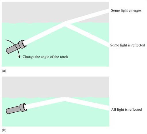
For comparison, take the torch out of the water and do the experiment the other way round, shining the beam into the water. In this case you should find that although as the angle gets smaller more of the light is reflected off the water surface, some light always enters the water. You do not get ‘total external reflection’.
While in principle optical fibre could use the boundary between the glass and air to contain the light – like you have demonstrated using the boundary between water and air – in practice the performance is very much better when using the boundary between the core and cladding glass, which can be controlled more accurately and is protected from damage.
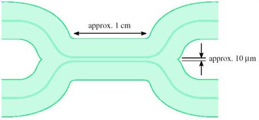
The basic types of optical fibre are single-mode and multimode, and are sketched in cross-section in Figure 3. Multimode fibre has a larger diameter core than single-mode, and, in simplistic terms, multimode fibre allows many different light paths (‘modes’) whereas single-mode allows only one. The significance of this difference will become clearer later.
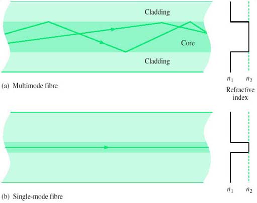
This idea of the modes in a fibre being different paths that rays can follow is known as the ‘ray model’ of light propagation. The model is useful for a qualitative understanding of the propagation of light in fibre, and can even be used for some quantitative analysis, but a complete understanding of light in fibre requires consideration of the electromagnetic fields.
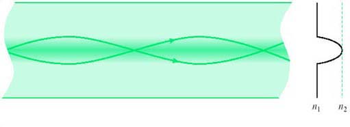
Both the fibres drawn in Figure 3 are what is known as step-index fibres, because the refractive index changes from core to cladding in a single step (abruptly). An alternative construction used for multimode fibre is graded-index (Figure 4), in which the refractive index varies smoothly from a maximum down the fibre axis to a minimum in the cladding. There are advantages to using graded-index fibre rather than step-index multimode fibre which will be considered later, and the fibre used for telecommunications purposes is nearly always either single-mode fibre or graded-index multimode fibre.
There are three types of fibre widely used for telecommunications (all three types have the same cladding diameter of 125 μm):
Single-mode step-index fibre with a cladding diameter of 125 μm and a core of about 10 μm. Specifications for fibres of this type are to be found in IEC 60793-2-50:1992 type B1 and ITU-T G.652, G.653, G.654 and G.655 (see References).
Multimode graded-index fibre with a cladding diameter of 125 μm and a core of about 50 μm. Specifications for fibres of this type are to be found in IEC 60793-2-10:1992 type A1a and ITU-T G.651.
Multimode graded-index fibre with a cladding diameter of 125 μm and a core of about 62.5 μm. Specifications for fibres of this type are to be found in IEC 60793-2-10:1992 type A1b.
The IEC specifications are generally used in LANs, and the ITU-T specifications for transmission in the core network. The differences between the several ITU-T specifications for single-mode fibre are to do with their dispersion characteristics, and are discussed later in Section 2.4.
Broadly speaking, the 10/125 μm single-mode fibre has the highest performance but is the most difficult to use, because the small core makes joints more difficult (notice the way of describing the fibre by ‘core-diameter/cladding diameter’, such as ‘10/125 μm’. Later I shall abbreviate further, referring to ‘10 μm’ fibre). The 50/125 μm multimode fibre is easier to use but has inferior performance (higher loss and smaller usable bandwidth). The 62.5/125 μm multimode fibre is the easiest to use but has the lowest performance. The characteristics of 50/125 μm and 62.5/125 μm fibre are quite similar, however, and in practice the difference tends to be just that the former has been used in Europe and the latter in the USA.
SAQ 3
These days telecommunications transmission in the core network invariably uses 10/125 μm single-mode fibre whereas LANs have mostly used one of the two multimode fibres. Why do you think this is?
Answer
Transmission systems in the core network need to transmit over longer distances than is needed in LANs, so the lower loss of single-mode fibre is a particular advantage, and it is worth the extra difficulty in using single-mode fibre. Because LANs do not involve such long distances, it is simpler to use multimode fibre. Note however that Gigabit Ethernet and 10 gigabit Ethernet have options for using single-mode fibre.
2.3 Attenuation
Activity 2
At approximately what wavelength is the attenuation of optical fibre lowest? What, approximately, is the attenuation at that wavelength? What other wavelengths are used and why?
Answer
The attenuation of fibre is lowest in the wavelength range 1500 to 1600 nm, where it is typically around 0.2 dB km−1. This is known as the ‘1500 nm window’, or more accurately the ‘1550 nm window’. Wavelengths around 1300 nm are widely used, however, because the dispersion of standard single-mode fibre is lower around 1300 nm and because optical devices are easier to manufacture at that wavelength (and are therefore cheaper). The attenuation in the 1300 nm region is still very low, being less than 0.5 dB km −1.
Wavelengths around 850 nm are also used because devices are even cheaper at that wavelength. For short distances (such as in LANs) the higher attenuation at 850 nm is still acceptable.
In order to determine the distance achievable with a given system, a link power budget is calculated. I shall illustrate this with examples based on Gigabit Ethernet standards. The material that follows refers to the IEEE 802.3 standard, 2002 edition.
The Gigabit Ethernet standards describe the use of fibre in all three categories identified in the last section. Two different versions of 50/125 μm multimode fibres are specified, differing in their bandwidth. Here I am talking about the version with a bandwidth specified by the ‘bandwidth-distance product’ of 400 MHz-km. (The meaning of the bandwidth-distance product is explained later.)
The 1000BASE-SX standard (‘S’ for ‘short wavelength’) specifies operation over either 50/125 μm or 65/125 μm multimode fibres using an optical wavelength of 850 nm. Consider first operating over 50/125 μm multimode fibre and the parameters of Table 1, which have been selected from the IEEE 802.3 standard.
| Parameter | Value |
|---|---|
| Minimum launch power | −9.5 dBm |
| Receive sensitivity | −17 dBm |
| Allowance for connector and splice losses | 1.5 dB |
| Maximum fibre attenuation | 3.5 dB km−1 |
| Link power penalties | 4.1 dB |
The minimum launch power and the receive sensitivity (the minimum power level required at the receiver) are requirements for the terminal equipment. The value for the maximum fibre attenuation is a requirement of the fibre used in the link, while the allowance for connector and splice losses and the ‘link power penalties’ are additional losses that need to be included. Several factors contribute to link power penalties, defined in paragraph 1.4.157 of IEEE 802.3 as follows:
1.4.157 link penalties: For fiber optic links, the power penalties of a link not attributed to link attenuation.
These power penalties include modal noise, relative intensity noise (RIN), intersymbol interference (ISI), mode partition noise, extinction ratio, and eye-opening penalties.
You do not need to know the details of these power penalties, but in general terms modal noise, RIN and mode partition noise are all effects due to features of the light source (in some cases also of the fibre). ‘Eye opening’ is to do with the tolerance to noise and jitter at the receiver, the concept of the data ‘eye’ coming from the appearance of the received signal when inspected with an oscilloscope.
With this information we first note that between the transmitter and receiver the maximum loss can be:

Notice that the difference between the two powers in dBm is in decibels, dB, not dBm, as it is a power ratio rather than an absolute power.
From this 7.5 dB we subtract the 1.5 dB allocated to the connectors and splices (splices are permanent joints between fibres, discussed further in Section 2.6) and 4.1 dB power penalties, leaving 1.9 dB for the fibre attenuation. This allows a length of 1.9/3.5=0.54 km (540 m). For this type of fibre the standard specifies an operating distance of up to 500 metres.
SAQ 4
Another of the Gigabit Ethernet standards, 1000BASE-LX, is specified for use with ‘long’ wavelengths (the ‘1300 nm window’) and can be used with single-mode as well as multimode fibre (50 μm and 62.5 μm). Using the data in Tables 2 and 3, draw up power budgets to determine the maximum range for 1000BASE-LX systems over:
(a) 50 μm multimode fibre
(b) 10 μm single-mode fibre.
Answer
(a) For the 50 μm system, the maximum loss between the transmitter and receiver can be:

1.5 dB of this available power budget is used by the connectors and splices and 5.0 dB for link power penalties, leaving 1.0 dB for the fibre attenuation. This allows a length of not more than 1.0/1.5 = 0.67 km, or 670 m. The standard specifies an operating distance of up to 550 metres.
(b) For the 10 μm single-mode system, the maximum loss between the transmitter and receiver can be:
1.5 dB of this available power budget is used by the connectors and splices and 3.3 dB for link power penalties, leaving 3.2 dB for the fibre attenuation. This allows a length of 3.2/0.5 = 6.4 km. The standard specifies an operating distance of up to 5 km.
| Parameter | Value |
|---|---|
| Minimum launch power | −11.5 dBm |
| Receive sensitivity | −19 dBm |
| Allowance for connector and splice losses | 1.5 dB |
| Maximum fibre attenuation | l.5 dB km1 |
| Link power penalties | 5.0 dB |
| Parameter | Value |
|---|---|
| Minimum launch power | −11 dBm |
| Receive sensitivity | −19 dBm |
| Allowance for connector and splice losses | 1.5 dB |
| Maximum fibre attenuation | 0.5 dB km1 |
| Link power penalties | 3.3 dB |
When referring to the wavelength of light in the context of optical-fibre communications it is the convention to refer to the wavelength that the light has in free-space.
2.4 Pulse spreading and bandwidth
Activity 3
Calculate the maximum signalling rate given by the Nyquist rate for the 1550 nm window, assuming that it runs from 1450 nm to 1610 nm.
Answer
Using the exact method from Section 1.2, the bandwidth is:
So the Nyquist rate is 4.12 ×10¹³ baud, or about 41 Tbaud.
This activity accurately portrays the massive potential capacity of optical fibre, but in practice it is not possible to exploit the full capacity directly – binary modulation at terabaud rates is a long way off!
In practice, the usable signalling rates in fibre are limited either by the speed at which the electronics at the transmitter and receiver can operate (at the time of writing, state-of-the-art commercial systems operate at up to 40 Gbaud) or by effects in the fibre that cause pulses to spread as they propagate along the fibre. Pulse spreading limits the maximum signalling rate because the more that pulses spread the more inter-symbol interference (ISI) you can get, and so the further apart in time symbols must be to prevent them interfering with each other. The amount of pulse spreading is proportional to distance – if pulses are spread by 1 ps (picosecond, 10−12 s) when travelling through 1 km of fibre then they will spread 2 ps over 2 km – so there is a trade-off between the usable bandwidth of fibre and the fibre length.
Actvity 4
Suppose a fibre spreads pulses at the rate of 200 ps km−1. What, approximately, is the maximum signalling rate that can be used with this fibre over a distance of: (a) 1 km, (b) 10 km?
Answer
Over 1 km the pulses spread by 200 ps and over 10 km they spread by 2 ns. You have to make some modelling assumptions about the pulses and at what point spreading will cause errors, but a starting point might be that the spreading must be less than half the symbol period, τ = 1/S, where S is the signalling rate. Over 1 km then, 0.5 × 1/S = 200 ps, so S = 0.0025 ×1012 = 2.5 Gbaud, and over 10 km we have S = 250 Mbaud.
A more complete analysis would take account of the fact that pulses don't remain rectangular as they spread, and that the effects are statistical – the error rate increases with increasing pulse spreading. The simple model of allowing spreading by up to half a symbol interval is adequate for order-of-magnitude considerations, however.
The main causes of pulse spreading differ between multimode and single-mode fibre, and will be considered next.
2.4.1 Multimode distortion
With multimode fibre, the main cause of pulses spreading is the multiple paths that signals can traverse as they travel along the fibre. This phenomenon of multimode distortion is illustrated in Figure 5.
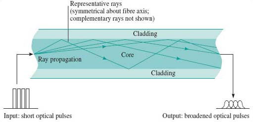
In the step-index fibre the light in the propagating modes is always in the core and therefore always propagating in glass with the same refractive index. The higher-order modes (the ones zig-zagging most) travel the furthest and therefore take the longest to propagate. In graded-index fibre the higher-order modes are in glass with a lower refractive index when they are off the axis. Light travels faster where the refractive index is lower, so in the graded-index fibre the light travels faster in the modes with the longer paths. This results, ideally, in the same overall propagation delay for all modes. A perfect balance is never possible, however, so there is still some pulse spreading due to multimode distortion even in graded-index fibre.
Spreading due to multimode distortion limits the usable bandwidth of a fibre. Since the amount of spreading is proportional to distance, the bandwidth is inversely proportional to distance, and the multimode distortion of a fibre is usually specified by the bandwidth-distance product.
Thus, for example, a 50/125 μm step-index fibre might have a bandwidth-distance product of 20 MHz·km. A 1 km fibre would have bandwidth of 20 MHz and a 2 km fibre would have a bandwidth of 10 MHz.
Activity 5
There are two different 50 μm graded-index multimode fibres specified for use with Gigabit Ethernet. Used with a 850 nm source, they are specified with a bandwidth-distance product of 400 MHz·km and 500 MHz·km. (The earlier discussion of power budgets considered only the first of these two.)
Given that the signalling rate of Gigabit Ethernet is 1.25 Gbaud, what will be the maximum fibre length for each of these fibres before bandwidth becomes a problem?
The signalling rate, 1.25 Gbaud, is higher than the data rate, 1 GHz, because of the line coding. The line coding is 8B10B, which means that for every 8 bits there are 10 binary symbols, so the signalling rate is greater than the data rate by a factor 10/8.
Remember that to avoid inter-symbol interference the maximum signalling rate that can be transmitted through a channel of bandwidth B is the Nyquist rate of 2B.
Answer
The minimum bandwidth is half the signalling rate, which is 625 MHz. The maximum lengths that will give this bandwidth are:
(a) the maximum distance is 400/625 = 0.64 km, or 640 m
(b) the maximum distance is 500/625 = 0.8 km, or 800 m.
In practice the bandwidth is not a sharp cut-off, and there would be some degradation to the signal for distances shorter than this. In fact, the degradation caused by multimode distortion is one of the sources of the link power penalty used in the calculation of the power budget earlier. In the Gigabit Ethernet standard the link power penalty for the 400 MHz·km fibre is 4.1 dB, but only 3.6 dB for the 500 MHz·km fibre, and the operating distance specified for the 500 MHz·km fibre is 550 m compared to 500 m for the 400 MHz·km fibre.
SAQ 5
1000BASE-SX over 62.5 μm multimode fibre is also specified for two different fibre bandwidth-distance products (Table 38-12 of IEEE 802.3):
(a) 160 MHz·km
(b) 200 MHz·km.
What will be the maximum fibre length before bandwidth becomes a problem with each of these fibres? (Remember that the signalling rate in Gigabit Ethernet is 1.25 Gbaud.)
Answer
The maximum lengths that will give a bandwidth of 625 MHz are:
(a) the maximum distance is 160/625 = 0.256 km, or 256 m
(b) the maximum distance is 200/625 = 0.320 km, or 320 m.
The standard specifies the operating distances as 220 and 275 m respectively.
Multimode fibre also suffers from dispersion as discussed in the following section, but multimode distortion is usually much greater than dispersion.
Note that you might sometimes see multimode distortion called multimode dispersion, but it is better to reserve the word ‘dispersion’ for spreading as a function of frequency, in the way described next.
2.4.2 Dispersion in single-mode fibre
Because there is only one mode in single-mode fibre, there is no multimode distortion but pulses are spread by dispersion.
Dispersion is the effect of different frequencies propagating at different speeds, and there are various mechanisms in optical fibre which mean that in general a fibre is dispersive. Given that dispersion takes place, a transmitted pulse will be spread because different frequency components in the pulse will take different lengths of time to propagate.
Activity 6
The spectrum of a modulated optical signal will always contain a range of frequencies. Why?
Answer
There are two reasons. First, the optical source has an inherent spectral width, as was discussed in Section 2.1 above. Second, even assuming an ideal optical source with a single frequency (zero spectral width) the modulation will spread the spectrum.
The pulse spreading due to dispersion has the effect of limiting the bandwidth of single-mode fibre in a similar way to that in which multimode distortion limits the bandwidth of multimode fibre. Dispersion, however, is usually described explicitly by the time-spread that it imposes on a pulse, using a parameter with units ps nm−1 km−1. The ‘nm’ (nanometres) in this refers to the spectral width of the optical source and the ‘km’ (kilometres) the length of the fibre. The ‘ps’ is the time-spread in picoseconds. Thus, for example, a light-emitting diode might have a spectral width of 40 nm (for example it might contain wavelengths in the range 1300 nm to 1340 nm) so that when used with a fibre with dispersion of 15 ps nm−1 km−1 the pulse will be spread by 40 × 15 = 600 ps for every kilometre of fibre. If the system is operating at 100 Mbaud then each symbol is 10 ns long and we might expect to run into problems if pulses are spread so that they approach about half of this, 5 ns, which happens when the fibre length is
SAQ 6
Laser diodes have much smaller spectral widths than LEDs. Depending upon the type of laser diode, the spectral width might be a few nanometres or much less than one nanometre. Suppose the system just described (i.e. operating at 100 Mbaud and using fibre with dispersion of 15 ps nm−1 km−1) uses a laser diode with a spectral width of 0.8 nm, how long can the fibre be in that case, before dispersion becomes a problem?
Answer
Pulse spreading will be 0.8 × 15 = 12 ps per kilometre, so there will be problems if the distance approaches
The magnitude of dispersion in single-mode fibre varies with wavelength and in standard single-mode fibre (as specified by ITU-T G.652) the dispersion is lowest at frequencies in the 1300 nm window (it takes on the value of zero at some value in this window) and much higher (of the order of 20 ps nm−1 km1) in the 1550 nm window. When the frequencies in the 1300 nm window were used for long-distance communications (in the 1980s and early 1990s) this was very convenient, but with the advent of optical amplification by EDFAs (erbium-doped fibre amplifiers) the 1550nm window became increasingly important and the high dispersion at those wavelengths became a problem.
The use of amplifiers, furthermore, at the same time as forcing a move to the higher-dispersion 1550 nm window, actually led to a demand for lower dispersion. Previously, before amplifiers were available, transmission links contained electrical regenerative repeaters. At appropriate intervals the signal was detected, converted to an electrical signal, regenerated, then converted back to an optical signal. Because of the regeneration, the signal transmitted on each repeater segment started off ‘perfect’, and in principle you could add more and more repeater sections indefinitely. (This is not quite true because regeneration is never perfect.)
Optical amplifiers, however, amplify the signal without regenerating it. So if you replace the regenerative repeaters with EDFAs, the pulse spreading due to dispersion carries through the amplifiers, and for the link to work correctly you need to consider pulse spreading over the whole end-to-end link. Whereas previously dispersion only had to be low enough to prevent errors over the length of a repeater section, now it has to be low enough to prevent errors over the length of the whole end-to-end link.
The technology of fibre design came to the rescue, however, because new fibres were developed in which the dispersion zero was shifted to the 1550 nm window. This type of fibre is known as dispersion-shifted fibre (DSF), and the ITU-T have specified such a fibre in recommendation G.653.
Instead of avoiding dispersion with low-dispersion fibre, it is possible instead to ‘undo’ dispersion through the use of dispersion compensation techniques. The basic principle of this is that you include in the optical path some component that has the exact opposite dispersion characteristic of the fibre path (Figure 6).
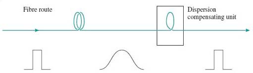
In particular, it is now possible to manufacture optical fibre with reversed dispersion characteristics. Thus, for example, if the refractive index of standard fibre is higher at 1551 nm than at 1550 nm, the dispersion compensating fibre has a refractive index that is lower at 1551 nm than at 1550 nm. Dispersion compensation is complicated to implement, but it allows existing fibre (standard single-mode fibre already installed) to be used with new systems. Furthermore, as will be seen later when we discuss fibre non-linearities, there are reasons why performance can be better over a system that uses dispersion compensation instead of zero-dispersion fibre.
2.4.3 Polarization mode distortion
Because light is an electromagnetic wave, it has a ‘state of polarization’, which, for light in single-mode fibre, is at right angles to the path of the fibre. If you've not encountered electromagnetic waves before, all you need to appreciate is that as light travels down the fibre the electromagnetic field has an orientation across the fibre (Figure 7). If it helps, you can imagine the light as a beetle crawling inside a hollow fibre, and the state of polarization as the orientation of the beetle in the fibre! (Figure 8)
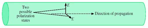
In a perfect fibre, the state of polarization has no effect on the propagation. But fibres are not generally perfect – for example, the core might not be perfectly circular or there might be stress across the fibre. In that case the speed of propagation of the light depends on the state of polarization. For a slightly oval core, for example, the velocity of propagation will be different for light polarized in the widest direction compared to the narrowest direction. (Perhaps the beetle can crawl faster if the tube is wide and low than if it is narrow and high.)
For this imperfect fibre, it is necessary then to consider two polarization states with different velocities as two polarization modes. Light can travel in both modes, and because they have different velocities the existence of these two modes leads to pulse spreading and distortion, in essentially the same way as multimode distortion. (The beetle analogy is a bit stretched now. You have to imagine two beetles setting off together, one crawling across the widest direction and one across the narrowest. One beetle gets to the end before the other.)
This is known as polarization mode distortion, PMD. (PMD is also used as an acronym for polarization mode dispersion, but as explained above concerning the use of the term ‘multimode dispersion’, it is better to keep the word dispersion for effects that are frequency-dependent.)
PMD is generally very small and has only become significant as systems operating at 10 Gbit/s or 40 Gbit/s have started to appear.
2.5 Non-Linearity
A linear system can be defined in two ways: (1) one which obeys the principle of superposition, and (2) one possessing the frequency-preservation property.
If we consider an optical fibre with electromagnetic field as the input and output, then provided that the power level of the input signal is not too great (less than 1 mW, which is 0 dBm), the fibre may be well modelled by a linear system for most purposes.
When fibre is used for a single point-to-point link to convey a digital signal by on-off keying, it is not too serious if the fibre does not behave precisely as a linear system. When fibre is used in a more sophisticated way, however, linearity becomes important. When using wavelength division multiplexing (WDM), for example, superposition is important.
Activity 7
What might happen if the fibre carrying WDM signals does not behave as a linear system?
Answer
If superposition does not hold in the fibre, one consequence is that the presence of one signal on the fibre will affect the output of the other signal, so there will be crosstalk between the signals. There will also be new frequencies generated by the interaction between different frequencies on the fibre.
When the power levels in the fibre increase significantly above 0 dBm, nonlinear effects can become significant, and this is an important consideration in dense wavelength division multiplexing. Note that the degree of non-linearity depends upon the total power in the fibre, and adding more wavelength channels also increases the power and therefore increases the amount of non-linearity.
Dense wavelength division multiplexing, DWDM, is WDM with closely-spaced wavelengths.
Non-linearity is not always ‘bad’ however, and in fact non-linearity is exploited in optical amplifiers as discussed in Section 3.3.
There are several different types of non-linearity in optical fibre. You do not need to know much about them for this unit, but it is useful if you have met the names. You should appreciate that they all refer to non-linear effects in fibre, and that they become more significant at higher power levels.
In summary, the most important ones are:
self-phase modulation, SPM
cross-phase modulation, XPM
stimulated Brillouin scattering, SBS
four-wave mixing, FWM
stimulated Raman scattering, SRS
Of these, four-wave mixing (FWM) in particular was found to have potentially serious consequences for dense wavelength division multiplexing, and stimulated Raman scattering is important because it is the process behind Raman amplifiers (discussed later).
Four-wave mixing is an effect in which light at different wavelengths interacts to generate light at another wavelength. The effect is characterised in terms of the frequencies of the waves, and in general light at four frequencies are involved: f1, f2, f3 and fnew. The light with the three frequencies f1, f2 and f3 interact due to non-linearities in the refractive index and generate light at the new frequency, fnew where
However f2 can be the same as f1 so that four-wave mixing involving only three different frequencies is possible. In this case:

It would be misleading to call this ‘three-wave mixing’ even though there are only three frequencies involved, because the frequency relationship involves four terms. Notice that all four terms can be closely spaced (e.g. they could all be optical frequencies in the 1550 nm window). If you had only three terms, one of the frequencies would have to be substantially different from the other two. Thus if fnew = f1 − f3 and f1 is close to f3, then fnew is much smaller than either of f1 or f3. This effect, where a new, much lower, frequency is generated by the difference between two closely-spaced frequencies, is called beating. Beating can be a problem at receivers where two closely-spaced optical signals can generate a new electrical signal at the beat frequency. I do not wish to consider beating any further, however, and return now to the discussion of four-wave mixing.
Four-wave mixing is damaging to DWDM signals for two reasons: it attenuates the signals and it introduces new signals which can cause interference.
For FWM to be significant in fibre it is necessary for the phase relationship between the various light signals to remain constant over long distances. This occurs if the dispersion is low, so, ironically, FWM in the 1550 nm window is worse in G.653 dispersion-shifted fibre than in standard G.652 fibre.
Activity 8
There was another way of reducing the effects of dispersion – an alternative to using fibre with a low dispersion coefficient – that was described earlier. What was it?
Answer
It is possible to use dispersion compensation.
It is possible therefore to reduce pulse spreading due to dispersion as well as avoiding the problems of FWM by using standard single-mode fibre combined with dispersion compensation.
A solution which avoids the need for dispersion compensation is to use fibre which has low but not zero dispersion in the 1550 nm widow. This is the reason for another single-mode fibre specified by the ITU-T G.655 standard – non-zero dispersion-shifted fibre (NZ-DSF).
Raman scattering (C. V. Raman, Indian physicist (1888–1970)) is a process in which light is scattered by the material through which it propagates, but in the process it changes its wavelength – specifically, the wavelength gets longer. In stimulated Raman scattering (SRS) light at the longer wavelength is already present in the medium, and increases (stimulates) the scattering. The ‘pump’ light is injected at the amplifier to provide a source of power for the amplification process. This is considered further in Section 3.3. In fibres carrying DWDM, SRS has the effect of transferring power from channels at shorter wavelengths to channels at longer wavelengths.
SAQ 7
What is dispersion-shifted fibre, and why has it become necessary in recent years when standard single-mode fibre was previously considered adequate?
Under what conditions is non-zero dispersion-shifted fibre preferable to dispersion-shifted fibre?
Answer
Standard single-mode fibre has the minimum dispersion in the 1300 nm transmission window. Dispersion-shifted fibre has the dispersion minimum shifted to the 1550 nm window.
Dispersion limits the bandwidth of single-mode fibre, so for high signalling rates low dispersion is required. The highest signalling rates can therefore be used at the wavelengths near the dispersion minimum.
Previously, the wavelengths used for transmission were in the 1300 nm window, which is therefore compatible with high signalling rates on standard single-mode fibre.
More recently the 1550 nm window has been used instead, because erbium-doped fibre amplifiers have been developed and these only operate around 1550 nm. Using standard single-mode fibre the higher dispersion would significantly limit the signalling rate at 1550 nm, so dispersion-shifted fibre is used instead.
Although low dispersion is desirable to minimise pulse spreading, it can increase the problems caused by non-linear effects in the fibre. In particular, when dense wavelength division multiplexing (DWDM) is used on a fibre, four-wave mixing (FWM) can be a significant problem if the dispersion is very low. DWDM uses the 1550 nm window, so the requirement for higher dispersion to reduce FWM can be achieved by going back to using standard single-mode fibre. The problem of high dispersion then returns, but that can be overcome through the use of dispersion compensation.
Dispersion compensation is complex to implement, so an alternative, preferable, solution is to use non-zero dispersion-shifted fibre. This has low enough dispersion in the 1550 nm window to allow high signalling rates without the need for dispersion compensation, but the dispersion is high enough to prevent problems with FWM.
2.6 Connecting and splicing fibres
There are two different types of fibre joint that need to be considered: permanent splices (the equivalent of soldered or crimped connections on copper cables) and demountable connectors.
Splices are used along a route to allow a link to be built up from convenient lengths of cable. The lengths are typically 2 km. Fibre is manufactured in lengths longer than this, but, once put in a cable, lengths longer than 2 km are difficult to transport and lay. Splices are also used to repair breaks in fibres. Connectors are used at the interface of equipment (such as a repeater, amplifier or terminal) to the cable.
The basic aim of a fibre joint (splice or connector) is to allow light to pass from the core of one fibre to another, with as little loss or reflection as possible. This is made more difficult by the difficulty of aligning the two fibres accurately, given the small size of the core.
There are two classes of problem which lead to loss through a joint (referred to as insertion loss):
Those resulting from differences between two fibres being joined, possibly because of imperfections in the fibres (variations in core or cladding refractive indices, core or cladding diameters, ellipticity, eccentricity of core and cladding), see Figure 9.
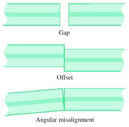
Those resulting from alignment error (gaps, offsets and angular misalignments of otherwise perfect fibres), see Figure 10. Because of the smaller core size, all of the above problems are more serious for single-mode than for multimode fibre.
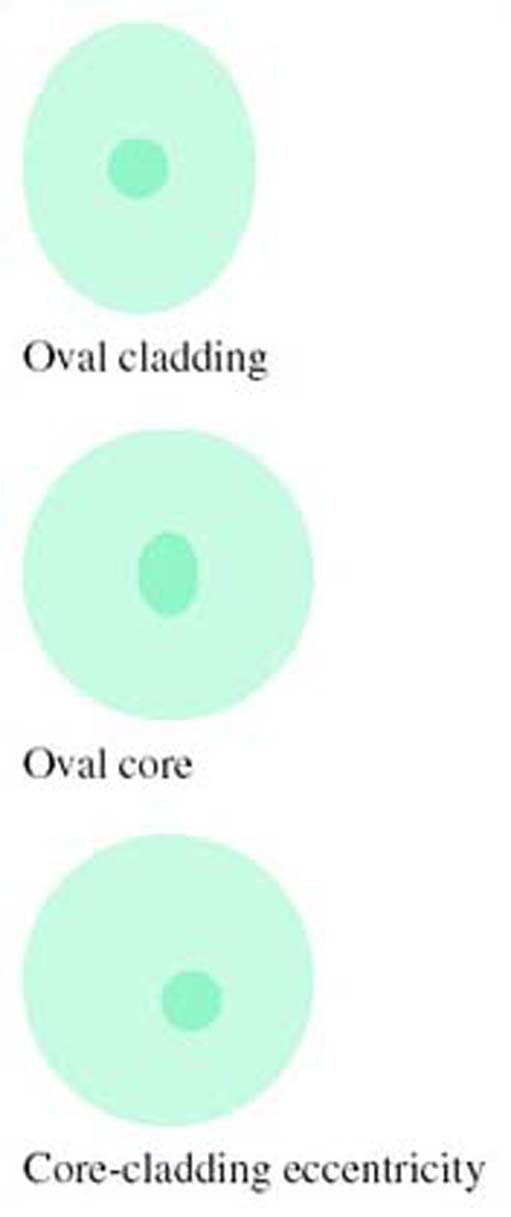
It might seem that, since the critical feature of a joint is aligning the cores, features of the cladding such as ellipticity or different diameters are unimportant, but this is not generally so. Most joints rely on using the outside surface of the fibre for alignment, so errors in the cladding can be transferred to a core misalignment. A method of alignment which avoids this problem is discussed in the section on splicing below.
As well as insertion loss, reflections at connectors can be a problem. Any sort of discontinuity in a fibre can result in some light being reflected back towards the source, so most connectors cause some reflection. (Splices can also cause reflection, but usually to a lesser degree.) In particular, if there is a gap between the ends of the fibres the abrupt change in refractive index between the glass and the air in the gap causes a reflection referred to as Fresnel reflection. From optical theory it can be shown that a step change in refractive index from n1 to n2 causes a fraction, r, of the light power to be reflected, where r is given by:

The refractive index of fibre used in communications-grade optical fibre is around 1.5, and the refractive index of air is about 1.0, so the Fresnel reflection between the fibre and the air is:
So around 4% of the light power will be reflected when the light enters the air gap, and 96% will enter the gap, Figure 11.

Activity 9
How much light will be reflected when the light enters the fibre at the end of the air gap?
Answer
The same fraction is reflected on leaving the gap as entering: 4%. This is 4% of the 96% that entered the gap, which is 0.04 × 0.96 × 100 ≈ 3.8% of the original light power (see Figure 11).
Activity 10
What, in dB, is the total insertion loss due to the two reflections?
Answer
The light power getting through to the far side of the gap is 0.96 × 0.96 × 100 ≈ 92.2%. In dB this, the insertion loss, is given by −10 log 0.922 = 0.35 dB.
Activity 11
What, in dB, is the ratio between the incoming power and the reflected power (the return loss)?
Answer
The total reflected power is 4 + 3.8 = 7.8% of the original power, so the return loss in dB is −10 log 0.078 = 11.1 dB.
This calculation neglects light paths that involve more than one reflection. These losses will be very small. (The power after two reflections is 0.04 × 0.04 × 100 = 0.16%.)
Reflection will only occur in this way if the gap is much bigger than the wavelength of the light being conveyed. If the gap is much smaller than the wavelength there will be little or no reflection. If the gap is similar in size to the wavelength then the nature of the reflection is complicated by interference effects and the amount of reflection depends upon the precise dimensions.
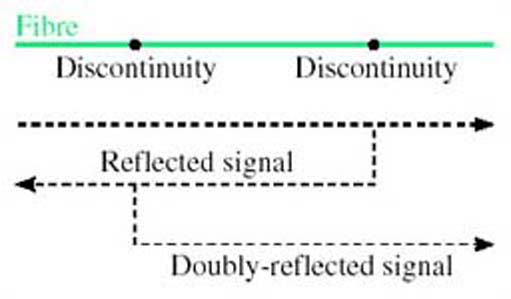
Reflected light can lead to increased noise on the signal from two effects. First, some lasers are sensitive to reflected light and become noisy or unstable when too much light is reflected back into them. Second, a double reflection (Figure 12) results in a delayed copy of the transmitted signal reaching the receiver. This delayed signal can result in an apparently disproportionately large amount of noise due to interference effects between the direct and reflected optical fields. Reflections are not normally a problem with splices, but techniques to minimise reflections have influenced changes in connector designs, as discussed influenced changes in connector designs, as discussed below.
SAQ 8
Suppose water intruded into the gap between two fibres. What fraction of power would be returned due to Fresnel reflections in that case? (Assume that the refractive index of water is 1.3.)
Answer
Using:
with n1 = 1.5 and n2 = 1.3 gives r = (0.2/2.8)2 = 0.0051, which is about 0.5%. This is the reflection from each surface (entering and leaving the gap), so the total reflection is about 1%.
The SAQ shows that the amount of reflection can be reduced by the presence in the gap of a material with refractive index close to that of glass. In practice water would not be used to do this – it would evaporate, for one thing. There are circumstance, however, where a special fluid or gel is used in the gap, which is designed to have the same refractive index as the glass and does not evaporate. This is index-matching fluid or index-matching gel.
2.6.1 Connectors
Many techniques have been used to design connectors that align the fibre ends accurately with high reliability and a long lifetime. The development of such components, at a low enough price, has been an important part of the overall development which has made fibre a feasible proposition for commercial transmission systems.
With fibre attenuation down to 0.2 dB km−1 (for single-mode fibre), the losses resulting from connectors and splices can be very significant over a whole route.
Activity 12
What length of fibre would have the same loss as the insertion loss due to the Fresnel reflections (0.35 dB) in a connector containing an air gap?
Answer
At 0.2 dB km−1, the loss due to the two Fresnel reflections in the connector is equivalent to 0.35/0.2 = 1.75 km of fibre.
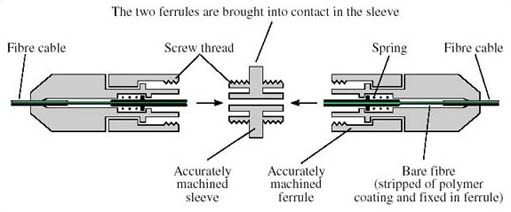
Figure 13 illustrates one type of connector, known as a ferrule connector (or FC connector).
In the basic connector the ends of the fibre are polished flat. In principle the two fibre ends could then abut, but any roughness on the surface (Figure 14), any dust on the fibre ends or any slight angular misalignment (Figure 10) will leave a gap between the cores. As noted above, if the gap is much less than the wavelength of the light being conveyed there is no problem, but since the wavelength is around 1.3 μm, this is a difficult target to meet.

Instead of polishing the ends flat, therefore, the ‘PC’ (physical contact) ferrule connector has the ends of the fibres polished to give two convex surfaces, resulting in better contact for the cores (Figure 15).

Even with the PC arrangement there is generally some residual reflection, and to minimise the reflections even further there is the angle-polished convex (APC) finish (Figure 16). (APC is sometimes taken to mean angled physical contact, but it still refers to the same method.) In this case the end-faces are polished at an angle, so that most of any light that is reflected is at an angle that is not guided by the fibre.

In general terms, PC connectors have the lowest insertion loss, whereas APC connectors have the lowest back reflections (APC is sometimes taken to mean angled physical contact, but it still refers to the same method.)
2.6.2 Splicing
The usual technique for splicing in the field is electric arc fusion splicing. This involves aligning the two fibre ends and then fusing them with an electric arc.
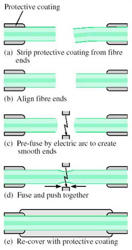
Specially designed jigs are used for this purpose, and the steps involved are as shown in Figure 17:
(a) Strip all protective coating from the fibre ends.
(b) Place the fibres on the jig and align the ends using a microscope.
(c) Pre-fuse the fibre ends to give a smooth surface.
(d) Bring the fibres together and fuse.
(e) Re-cover the stretch of bare fibre with a protective coating.
To avoid relying on the outside surface of the fibre for alignment, a technique is used in some jigs based upon shining light through the two fibres while they are being aligned. The best alignment is indicated by the lowest loss. Light injection and extraction is done (all within the jig) by bending the fibres beyond the point at which light is guided (Figure 18) – but not so far as to risk damaging the fibre.

2.7 Cabling
A distinction must be made between the optical fibre – a single strand of glass fibre – and the optical-fibre cable consisting of one or more strands of fibre and various protective coverings.
Bare optical fibre is fragile and vulnerable, and the cabling must provide the properties given below.
Tensile strength: The cable should prevent the fibre being strained when the cable is under tension. When the cable is being laid, for example, pulling it through a duct results in considerable tension.
Abrasion resistance: Abrasion on the surface of the fibre will weaken it significantly because cracks, starting at surface scratches, will readily propagate right across the fibre. The cable around the fibre must protect it from such abrasion.
Resistance to radial compression: There must be sufficient radial strength in the cable to shield the fibre from the expected radial force.
Bend resistance: If the fibre is bent such that its radius of curvature is less than a critical minimum, its attenuation starts to increase as a result of light loss. The cable must ensure that the fibre is never bent that severely.
Environmental protection (chemical resistance): Certain chemicals can react with the glass of the fibre to change its optical properties. For example, hydrogen can increase the attenuation. The cable must prevent such chemicals coming into contact with the fibre.
These are the principal characteristics required of the cable, but there are other hazards against which the fibre must be protected in particular circumstances. For example, frequent vibration or flexing of the fibre could weaken it so that it eventually breaks.
The first stage of protection of the fibre is the addition of one or more polymer layers as soon as the fibre is manufactured, before it is wound onto a drum. This is necessary to protect against abrasion, which can very easily damage the bare fibre. The polymer-coated fibre is then cabled to provide various degrees of protection depending upon the application. At one extreme the cabling could be just further plastic covering to produce a cable for use within a rack of equipment. At the other extreme many fibres could be put together in an armoured cable for use in a submarine optical-fibre link.
3 Optical components
3.1 Introduction
The basic optical-fibre link consisted of the source (laser or LED), the fibre and the detector, as was shown in Figure 1. Improvements in these components can increase the data rate, but the system is still a point-to-point transmission link and all signal processing, such as routeing, switching and regeneration, is done in electronics.
With the availability of devices that can process optical signals directly comes the possibility of using fibre in a more sophisticated way, leading eventually to an all-optical network.
This section considers some of the technology used and the components that have been created which might form the building-blocks of an optical network – or at least allow fibre to be used for slightly more than a point-to-point transmission link.
3.2 Directional couplers
A simple yet valuable device is the directional coupler (Figure 19). A directional coupler can be constructed from two single-mode fibres by bringing them into close contact and heating so that the glass melts and the two fibres fuse. Light can then pass from one fibre to the other.
A directional coupler constructed from fibres in this way is known as a fused fibre coupler.
Depending upon the details of the way directional couplers are made – how long the fused section is, how closely joined the fibres are – they can be made to have different properties for different purposes. For example, a ‘3 dB coupler’ is designed so that light entering from one fibre splits equally to the two fibres at the output.
Activity 13
Why do you think this is called a 3 dB coupler? Think about the ratio between the input and output power.
Answer
Since the input is split equally between the two outputs, the power on each of the outputs is half that at the input (assuming an ideal device). In decibels, the ratio between the input power and the output power is therefore 10 log(2) = 3 dB.
The question assumed an ideal component. Real optical components invariably have additional loss due to imperfections. This is called the excess loss. The overall ratio between the input and output power, expressed in decibels, is the insertion loss.
Another factor that might need to be considered in a real 3 dB coupler is the asymmetry between the two outputs, because the splitting might not be exactly equal between the two.
Activity 14
Suppose a nominally 3 dB coupler has an excess loss of 0.1 dB. What is its insertion loss?
Answer
The insertion loss is just the nominal loss plus the excess loss, 3.1 dB.
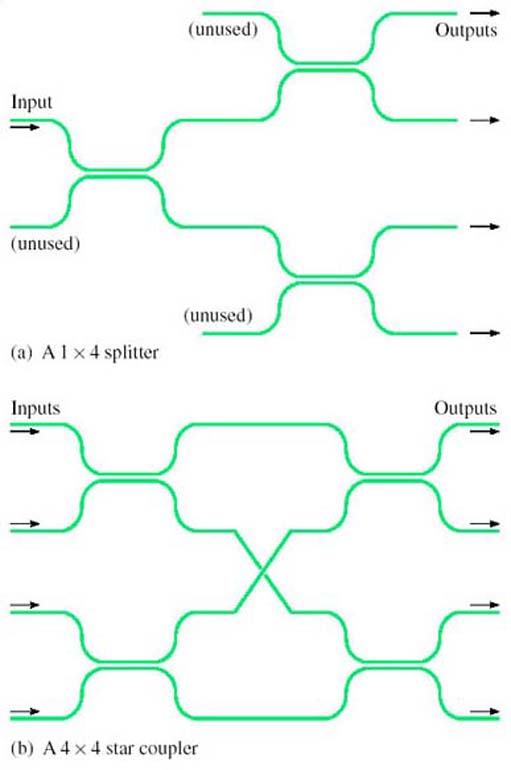
For some applications multi-way tree and star topologies are useful in fibre systems. Multi-way splitters and combiners (for the tree topology) and star couplers can be built from concatenated directional couplers as shown in Figure 20. Assuming the directional couplers are 3 dB couplers, the configuration in Figure 20(a) splits light equally to each of the four outputs. In the configuration in Figure 20(b) light on each of the four inputs is split equally to all of the four outputs – so the outputs each have light from all of the four inputs. Directional couplers work in both directions; so, for example, the splitter can also be used as a combiner. In Figure 20(a) one-quarter of the light entering any of the ‘outputs’ will reach the input. (It is only one-quarter, because the rest of the light goes to the fibres labelled ‘unused’.)
SAQ 9
Suppose a splitter is built from 3 dB couplers to distribute light to 16 outputs, and that each of the couplers has an excess loss of 0.2 dB. If the power on the input is −4 dBm, what is the power on each of the outputs expressed both in dBm and milliwatts?
Answer
Each coupler introduces a loss of 3.2 dB. The light has to pass through four couplers to get to an output (see Figure 21), so the loss is
4 × 3.2 = 12.8 dB
The power on the output is therefore
−4 − 12.8 = −16.8 dBm
This is 10−1.68 = 0.0209 mW, or about 21 μW.
As a check that this is about right, the power on the input is −4 dBm which is 10−0.4 = 0.4 mW. If the splitters were perfect this would be split equally 16 ways, so that the power on each output would be 0.4/16 = 0.025 mW. The excess loss reduces this to 0.021 mW.

In general, the properties of a directional coupler depend upon wavelength, and this can be useful. For example, a device can be constructed to combine or split two wavelengths, to perform wavelength division multiplexing.
3.3 Optical amplifiers
Figure 22 shows in outline one possible structure for an Erbium-doped fibre amplifier (EDFA).
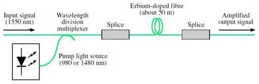
A length of erbium-doped fibre is spliced in line with the fibre carrying the signal, and high-power, unmodulated light at a specific, shorter, wavelength (the ‘pump’ wavelength) is coupled into the same fibre. The erbium-doped fibre has the same physical structure as standard single-mode fibre but the glass it is made of has erbium atoms added (it is ‘doped’ with erbium), and the presence of the erbium has the effect of transferring energy from light at the pump wavelength to the signal wavelength. In this way the (modulated) signal at around 1550 nm emerges from the erbium-doped fibre at a higher power, having taken the power from the pump.
The wavelength of the light used for the pump can be either 980 nm or 1480 nm. Sometimes both pump wavelengths are used simultaneously to get maximum gain.
While EDFAs are simple in principle and have had a dramatic effect on optical-fibre communications, there are a number of considerations that must be taken into account when they are used, including:
Cost: Both the wavelengths used in the pump source are difficult to generate and the lasers used to produce them are expensive.
Noise: In addition to amplifying the input signal, EDFAs (like all amplifiers) also generate a noise signal, in this case known as amplified spontaneous emission (ASE).
Gain-flatness: In an ideal amplifier a plot of gain against wavelength would be flat across the range of wavelengths for which it is to be used. In a real amplifier the gain depends to some extent upon the precise input wavelength. This can be a problem in systems carrying WDM (wavelength division multiplexed) signals since some wavelengths will be amplified more than others.
In addition, as already explained, EDFAs only work in the 1550 nm window.
Other technologies are available for manufacturing optical amplifiers. For example, semiconductor optical amplifiers (SOAs), also called semiconductor laser amplifiers (SLAs), can be made for use in both the 1550 nm and 1300 nm windows. They use the same technology as the laser diodes that provide the light source at the transmitter, but have a different physical structure. Although SOAs have been available for some time and are potentially cheaper than EDFAs, their performance is not as attractive as EDFAs and they have not been very widely used.
At the time of writing Raman amplifiers have just started to appear commercially. Raman amplifiers use stimulated Raman scattering (SRS) to transfer power from light at a pump wavelength to the signal. This effect is similar to what happens in an EDFA, but is caused by a different physical property leading to different characteristics. Whereas EDFAs transfer power from one or both of two specific pump wavelengths to a specific range of signal wavelengths, with SRS the importance lies in the difference between the pump wavelength and the signal wavelength. For both the 1300 and 1550 nm windows a pump at any wavelength will amplify light with a wavelength about 100 nm longer. Thus if you want to amplify light at, say, 1330 nm you need a pump with a wavelength of about 1230 nm. By having several pumps at different wavelengths, it is possible to amplify over a large range of signal wavelengths.
When considering optical amplifiers it is convenient to refer to the frequency ranges available for optical-fibre transmission defined by Ramaswami and Sivarajan (2002):
| O band | (O for ‘original’ wavelength band) | 1260–1360 nm |
| E band | (E for ‘extended’ wavelength band) | 1360–1460 nm |
| S Band | (S for ‘short’ wavelength band) | 1460–1530 nm |
| C Band | (C for ‘conventional’ wavelength band) | 1530–1565 nm |
| L Band | (L for.‘long’ wavelength band) | 1565–1625 nm |
| U band | (U for ‘ultra-long’ wavelength band) | 1625–1675 nm |
SAQ 10
What technologies can be used to amplify optical signals in the following bands?
(a) O band
(b) C band.
Answer
(a) Semiconductor optical amplifiers (SOAs) and Raman amplifiers can be used in the O band.
(b) Semiconductor optical amplifiers and Raman amplifiers can also be used in the C band, but additionally erbium-doped fibre amplifiers (EDFAs) can be used at these wavelengths.
3.4 Optical switches
Optical space switching has been possible for a long time, but has been slow to find widespread application.
Solid-state optical switching (i.e. switching with no moving parts) can use devices based upon electro-optic materials such as lithium niobate (LiNbO3). An electro-optic material is one whose refractive index changes significantly when an electric field is applied across it.
Figure 23 shows a 2 × 2 switch element which exploits the electro-optic effect. This is a coupler, similar to those previously described, but in the coupling region the light travels in an electro-optic material such as lithium niobate instead of glass. When an electric field is applied across one or both of the light paths, the amount of light crossing between the two paths changes.
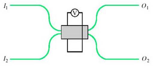
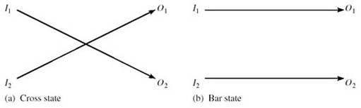
With suitable design, it can be arranged to switch between the ‘cross’ state (light entering I1 emerges from O2, and light entering I2 emerges from O1, as in Figure 24(a) and the ‘bar’ state (light entering I1 emerges from O1 and light entering I2 emerges from O2, as in Figure 24(b) under the control of the applied voltage, V.
Electro-optic switches such as these can be operated at high speed – switching between the two states can be as fast as 10 ps – but they are expensive, they generally introduce high losses in the optical signal (up to 8 dB) and can introduce distortion in the transmitted signal due to polarization effects.
A more recent development is the micro-electro-mechanical system switch. Micro-electro-mechanical systems (MEMS) are miniature electrically operated mechanical devices which can be constructed using the same materials and similar processing techniques as for large scale integrated electronic components. For optical switching, miniature movable mirrors can be made, each with dimensions of less than a millimetre. The movement of the mirrors can be controlled by an electrical signal, and incoming light beams from optical fibres can be directed to one of several different output fibres to perform the switching function.
With this technology, compact switching arrays with large numbers of crosspoints can be constructed as illustrated in Figure 25.
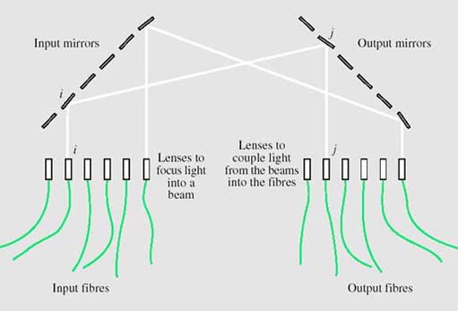
Two arrays of mirrors are used, one associated with the input fibres and one with the output fibres. Each of the mirrors on the input array can deflect the input beam to any of the mirrors on the output array. To switch from input fibre i to output fibre j, the mirror i on the input array deflects the beam from input fibre i to mirror j on the output array. Mirror j then deflects this beam to output fibre j.
Figure 25 shows a line of input and output fibres, but this is only to simplify the illustration. In practice the fibres (and mirrors) are in rectangular arrays, allowing more fibres to be packed into a small structure. They can be constructed with large arrays of crosspoints – typically 32 × 32 or 64 × 64 arrays, but up to 1000 × 1000.
Compared to switches based upon electro-optic materials, MEMS switches are slow (switching times of the order of 10 ms) but introduce less attenuation (of the order of 5 dB).
Because of the importance of optical switching, there has been a lot of research effort put into investigating different switch technologies, and the two presented here represent two extremes: fast, small arrays in the case of lithium niobate electro-optic switches and slow, large arrays in the case of MEMS switches. Lithium niobate electro-optic switches have been available for many years but have not yet been used commercially to any great extent. MEMS switches on the other hand have only been developed recently (2002) and are already starting to be exploited commercially.
3.5 Wavelength multiplexing and demultiplexing
Wavelength multiplexers and demultiplexers are needed in order to be able to use wavelength division multiplexing. With just two wavelengths, the multiplexers and demultiplexers can be based on directional couplers because, as mentioned earlier in Section 3.2, couplers are naturally wavelength-dependent and with appropriate design can be arranged to split and combine two chosen wavelengths. As shown in Figure 26, and using the language of a 2 × 2 switch (Figure 24), the coupler is in the ‘cross’ (over) state for λ2 and the ‘bar’ (non cross-over) state for λ1.

With dense wavelength division multiplexing (DWDM) forty or more wavelengths can share a single fibre.
A number of different technologies have been developed for multiplexing and demultiplexing multiple wavelengths, but the principle is illustrated by a prism, as shown in Figure 27. You are probably familiar with the way in which a prism splits white light into its constituent colours (the rainbow effect), so the principle can be used to separate the different wavelengths in the beam emerging from a fibre carrying a DWDM signal.
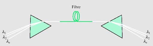
Used in reverse, a prism can combine the different wavelengths into a single DWDM beam. Wavelength division multiplexers and demultiplexers based upon prisms can be used in practice for DWDM, but not quite as drawn in Figure 27 because lenses are required to couple the light into and out of the fibres.
SAQ 11
Identify three uses of devices based upon directional couplers.
Answer
Three uses of devices based upon directional couplers:
Power splitting, such as for a tree topology
Constructed with electro-optical material, they can be used for switching
They can also be designed so that the splitting is wavelength-dependent so that they can be used as wavelength division multiplexers or demultiplexers.
4 Developments and future directions in optical-fibre communications
4.1 Introduction
Additional material for this unit, by David Chapman, January 2005
The start of optical-fibre communication is generally identified with a paper published in 1966 (Kao and Hockham, 1966). It was not until about ten years later that it was commercially viable, but from then on there was more or less continuous development, with substantial research effort taking place both in industry and universities.
Innovation continues today, and this additional material introduces some of the fields of development that are being pursued now.
A good overview of the history of optical-fibre communications in the UK can be found in a paper by Professor Midwinter of University College London, published in the ‘Millennium Issue’ of the IEEE Journal on Selected Topics in Quantum Electronics (Midwinter, 2000).
Coherent optical communications: a cul-de-sac?
In the 1980s, a lot of research effort was expended on developing a technique known as ‘coherent detection’ of optical signals. The technique involved applying to optical signals a method that is widely used in the detection of radio signals, but that is much more difficult to do with optical signals because of the very much higher frequency of light (of the order of 10 Hz) compared to radio (under 10 Hz). Coherent detection provides a way of building receivers with very high sensitivity, and might also be used to allow closer channel spacing in wavelength division multiplexed signals.
Previously, I wrote:
At the time of writing (1988), although coherent detection has been demonstrated in many impressive experiments, it still requires further development before it will be suitable for use in commercial optical systems
and
Full exploitation of the capabilities of optical fibre can be achieved by the use of … coherent detection.
As I write now, 18 years later, commercial deployment of coherent detection has still not taken place, and the research effort has tailed off. To a large extent, interest in coherent optical techniques waned with the development of erbium-doped fibre amplifiers (EDFAs). The main attraction, in the short term at least, of coherent detection was the very high receive sensitivity that it gave, which in turn was desirable because it allowed longer transmission distances between repeaters. Optical amplifiers provided the same benefit (long repeater spacing), and it turned out that EDFAs were much simpler to use than coherent optical detection. The use of coherent techniques in wavelength division multiplexing might still be valuable one day, but for the present other, simpler, technologies are sufficient and coherent optical techniques looks like a research avenue that turned into a cul-de-sac.
4.2 Fibre in the core network
All new trunk transmission – that is, transmission between telephone exchanges – is now over optical fibre. Mostly it uses either PDH or SDH links. Year by year the data rates have increased, so that at the time of writing STM-64 products are available commercially.
SAQ 12
What, approximately, is the bit-rate of an STM-64? What is the bit-rate of the next stage to be developed?
Although STM-256 systems are expected to be available soon, there are difficulties with operating them on currently installed fibre, and there are doubts that the trend of ever-higher time-division multiplexed rates will continue indefinitely.
Answer
An STM-64 will run at approximately 64 × 155.52 = 9953 Mbit/s, which is about 10 Gbit/s.
The SDH hierarchy increases by factors of 4, so the next stage is STM-256, at approximately 40 Gbit/s.
Activity 15
What are the problems with operating at ever higher data rates over single-mode fibre?
Discussion
As the data rates increase the tolerance to pulse-spreading decreases. At 40 Gbit/s, on single-mode fibre, dispersion and polarization-mode distortion significantly limit the transmission distance. (Multimode fibre could only be used for very short distance because of multimode distortion.)
The solution being used for increasing further the capacity of fibre is therefore wavelength division multiplexing, WDM.
In Recommendation G.671 the ITU-T identified three categories of WDM, defined by the spacing between the channels as follows:
You will see later that wide WDM, WWDM, is used to mean something rather different in the standard for 10 Gigabit Ethernet.
3.1.14.1 Coarse WDM (CWDM) device
A class of WDM devices having a channel wavelength spacing less than 50 nm but greater than 1000 GHz (about [X] nm at 1550 nm and [Y] nm at 1310 nm). Devices within this class can cover several spectral bands.
3.1.14.2 Dense WDM (DWDM) device
A class of WDM devices having a channel spacing less than or equal to 1000 GHz. Devices within this class can cover one or more spectral bands.
3.1.14.3 Wide WDM (WWDM) device
A class of WDM devices having a channel wavelength spacing greater than or equal to 50 nm. This device class typically separates a channel in one conventional transmission window (e.g. 1310 nm) from another (e.g. 1550 nm).
The mixtures of wavelengths and frequencies used in these quotes from the ITU standard is typical of the literature of optical-fibre communications: wavelengths used to describe the windows (e.g. 1310 nm and 1550 nm) and large channel spacings (e.g. 50 nm), but frequencies used for small channel spacings (e.g. 1000 GHz). Notice, though, that in the definition for CWDM it is technically incorrect to say ‘… channel wavelength spacing less than 50 nm but greater than 1000 GHz …’ because it is using the units of frequency (GHz) for a wavelength spacing. What it could say instead is ‘…channel wavelength spacing less than 50 nm but greater than a frequency spacing of 1000 GHz…’.
SAQ 13
The ITU specification for CWDM quoted above included the wavelength equivalents (in nm) of 1000 GHz at 1550 nm and 1310 nm, but I have replaced them by X and Y respectively. Use the appropriate formula to calculate X and Y.
Answer
The formula you need is:
The frequency spacing, Δf, is 1000 GHz (1012 Hz) and c, the speed of light (to three significant figures) is 3.00 × 10⁸ m s−1. For X, λ, is 1550 nm, so that the wavelength spacing is:
So X, the wavelength spacing in the 1550 nm window, is 8 nm.
For Y, λ is 1310 nm, so that the wavelength spacing is:
So Y, the wavelength spacing in the 1310 nm window, is 5.7 nm.
Early applications of WDM were of the WWDM type, used with directional couplers for the multiplexing and demultiplexing (with λ1 = 1300 nm and λ2 = 1550 nm).
The characteristics and applications of CWDM are summarised in ITU-T Recommendation G.694.2:
Coarse Wavelength Division Multiplexing (CWDM), a WDM technology, is characterised by wider channel spacing than Dense WDM (DWDM) as defined in G.671. CWDM systems can realise cost-effective applications, through a combination of uncooled lasers, relaxed laser wavelength selection tolerances and wide pass-band filters.
CWDM systems can be used in transport networks in metropolitan areas for a variety of clients, services, and protocols.
and those of DWDM in Recommendation G.694.1:
Dense Wavelength Division Multiplexing (DWDM), a WDM technology, is characterised by narrower channel spacing than Coarse WDM (CWDM) as defined in G.671. In general the transmitters employed in DWDM applications require a control mechanism to enable them to meet the application's frequency stability requirements, in contrast to CWDM transmitters which are generally uncontrolled in this respect.
The significance of the reference to ‘uncooled lasers’ is that in general the wavelength of light from a laser varies as the temperature changes. DWDM needs very stable wavelength sources, so the temperature of the lasers must be controlled. This is not necessary for CWDM.
Systems using DWDM generally also use optical amplifiers. Although DWDM can be used in links without amplifiers, it is the availability of amplifiers that has made DWDM so attractive. For one thing, wavelength multiplexers and demultiplexers tend to be quite lossy, so that without amplifiers the power budget available for the transmission path would be quite small. If a regenerative repeater were needed to extend the transmission distance it would have to demultiplex all the wavelength channels, detect each channel with a photodiode, regenerate each channel and then recreate the multiplexed optical signal. An optical amplifier, which amplifies all channels simultaneously, is much simpler.
ITU-T Recommendations G.694.1 and G.694.2 contain wavelength grids – tables of the wavelengths that should be used. The table for CWDM from G.694.2 uses 20 nm channel spacing and is reproduced in Table 5. For DWDM, G.694.1 recommends channels based on a grid spaced by 12.5 GHz (approximately 0.1 nm), as shown in Table 6. For systems using channel spacings of 25 GHz (approximately 0.2 nm) every alternate wavelength on the 12.5 GHz grid is used; for spacings of 50 GHz (approximately 0.4 nm) every fourth wavelength on the 12.5 GHz grid is used; and similarly for wider channel spacing.
| Nominalcentral wavelengths (nm) for spacing of 20 nm | |
|---|---|
| 1270 | 1450 |
| 1290 | 1470 |
| 1310 | 1490 |
| 1330 | 1510 |
| 1350 | 1530 |
| 1370 | 1550 |
| 1390 | 1570 |
| 1410 | 1590 |
| 1430 | 1610 |
Note: The end-points of this table are illustrative only.
| Nominal central frequencies (THz) for spacings of: | Approximate nominal central wavelengths (nm) | |||
|---|---|---|---|---|
| 12.5 GHz | 25 GHz | 50 GHz | 100 GHz and above | |
| 193.2375 | — | — | — | 1551.42 |
| 193.2250 | 193.225 | — | — | 1551.52 |
| 193.2125 | — | — | — | 1551.62 |
| 193.2000 | 193.200 | 193.20 | 193.2 | 1551.72 |
| 193.1875 | — | — | — | 1551.82 |
| 193.1750 | 193.175 | — | — | 1551.92 |
| 193.1625 | — | — | — | 1552.02 |
| 193.1500 | 193.150 | 193.15 | — | 1552.12 |
| 193.1375 | — | — | — | 1552.22 |
| 193.1250 | 193.125 | — | — | 1552.32 |
| 193.1125 | — | — | — | 1552.42 |
| 193.1000 | 193.100 | 193.10 | 193.1 | 1552.52 |
| 193.0875 | — | — | — | 1552.62 |
| 193.0750 | 193.075 | — | — | 1552.73 |
| 193.0625 | — | — | — | 1552.83 |
| 193.0500 | 193.050 | 193.05 | — | 1552.93 |
| 193.0375 | — | — | — | 1553.03 |
| 193.0250 | 193.025 | — | — | 1553.13 |
| 193.0125 | — | — | — | 1553.23 |
| 193.0000 | 193.000 | 193.00 | 193.0 | 1553.33 |
| 192.9875 | — | — | — | 1553.43 |
| 192.9750 | 192.975 | — | — | 1553.53 |
| 192.9625 | — | — | — | 1553.63 |
SAQ 14
In what band are the frequencies of Table 6? If the whole of this band could be filled with channels at 25 GHz spacing, how many channels in total would there be?
You will need to convert from wavelengths to frequency, using f = c/λ, where fis the frequency, λ (lambda) the free-space wavelength and c the speed of light, which, to six significant figures, is 2.99792 × 10⁸ ms−1.
If each channel carries an STM-64, what will be the total data rate carried by the fibre?
At the time of writing, commercial products are available that can support up to 160 STM-64 channels.
Answer
The wavelengths of Table 6 are all in the C-band.
The C-band extends from 1530 nm to 1565 nm, which is, in terms of frequency, from
to
This is a range of 195.94 − 191.56 = 4.38 THz, and at a spacing of 25 GHz (0.025 THz) per channel that would allow 4.38/0.025 = 175.2 channels. Rounding down, that would in practice be 175 channels.
If each channel carries an STM-64 this is a total capacity of approximately 175610 Gbit/s = 1.75 Tbit/s.
4.3 Optical networking
DWDM improves the utilisation of optical fibre for point-to-point links, but a further step in exploiting the potential of optical fibre comes from optical networking in which routeing or switching is done optically.
Optical networking is in its infancy, but the concept of the optical layer based upon wavelength channels is emerging. The optical layer effectively sits below the SDH layer in the network, and provides wavelength channels from one location to another.
An analogy can be drawn between networking with SDH and the optical network, where wavelength channels in the optical layer perform the equivalent function to containers in SDH. Then, as SDH transports containers across a network, so the optical layer transports wavelengths. A DWDM transmission link is the equivalent of an STM-n.
Activity 16
Can you think what function would be required of optical equivalents of cross-connects and add/drop multiplexers?
Discussion
Add/drop multiplexers would have to extract and replace individual wavelength channels, as in Figure 28 (a). Cross-connects would have to interconnect wavelength channels between different DWDM links, as in Figure 28(b).
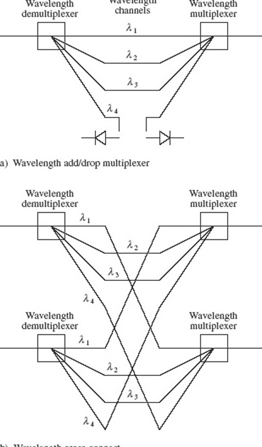
Activity 17
The space switching shown in Figure 28(b) can be done with MEMS switches (Figure 25), but the resulting cross-connect will not be as flexible as it might first appear. Can you see in what way it is limited, and what more is needed for full flexibility?
Discussion
Incoming wavelengths have to go to the same wavelength channels in the output, as it stands. For a fully flexible switch, wavelength conversion is needed. (It is like being able to do time-multiplexed space switching of PCM channels, but not being able to do time switching.)
It is possible to perform wavelength conversion by going via an electrical signal – detecting the optical signal at one wavelength and generating another optical signal at a different wavelength. More flexibility then comes from having wavelength-tunable lasers. An ‘all-optical’ device would be preferable, however, and experimental devices exist that can do this, but wavelength converters are perhaps the least-developed devices that are required for a universal optical layer.
4.4 Fibre in the access network
In the 1980s there was a belief that it was only a matter of time before fibre would be installed in the access network (from individual private customers to the local telephone exchange, also called ‘the last mile’, the ‘local loop’ and, now, the ‘first mile’). Installing ‘fibre to the home’, FTTH, as this has come to be known, was always recognised to be a major undertaking, simply because of the number of links involved. If, however, the revenue from new services enabled by the large bandwidth of optical fibre is sufficient, then telecommunications operators would be able to finance the development. Over the years, therefore, operators have looked for bandwidth-hungry ‘killer applications’ that might justify FTTH. For a while it was hoped that ‘video on demand’ would fulfil that role, and now with the expansion of the Internet there is increasing demand for broadband Internet access. Though there have been a number of trials with FTTH, to date none of them has demonstrated that it is a commercial proposition.
4.4.1 FTTCab, FTTC, FTTB and hybrid coaxial fibre
The equipment needed at optical-fibre transmitters and receivers (lasers, photodiodes and the associated electronics) is more expensive than the equivalent for transmission over copper cables. With FTTH this equipment is needed in every home, and a substantial cost reduction is possible with schemes where the fibre doesn't go all the way to the home, but stops short, and copper links run from a shared fibre to several homes (Figure 29). This is the basis of several schemes, such as fibre to the cabinet, FTTCab.
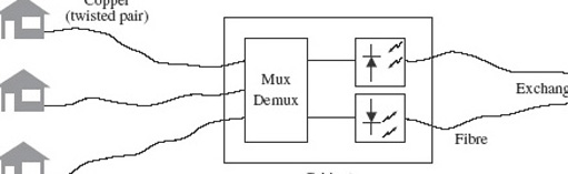
Typically in FTTCab the signals for all the attached houses are multiplexed onto a single fibre (or rather a pair of fibres, one for each direction of transmission) and equipment in the street cabinet performs conversion between the electrical and the optical signals as well as multiplexing and demultiplexing. FTTCab exploits the capacity and low attenuation of fibre while only needing a single pair of optical transmitters and receivers shared between several houses (maybe tens or even hundreds of houses might share the one fibre), and links from the cabinet to the houses would typically use twisted-pair cables.
FTTC is fibre to the curb/kerb (where ‘curb’ is the US spelling of ‘kerb’), and is really the same as FTTCab but taken closer to the homes, so that each fibre serves fewer houses. The split is done in a hub located on the kerb to serve the nearby houses.
FTTB, fibre to the building, goes further, taking the fibre into a building, but the building is typically a block of flats or some other shared building and the drop to the individuals is over copper, as with FTTCab and FTTC.
FTTX
All these acronyms beginning FTT, which are to do with getting fibre closer to the user, are sometimes grouped together under the heading ‘FTTX’ – with the ‘X’ as a sort of variable that can be B, C or whatever. They are not at all standardised and authors tend to pick any that suits them at the time. A colleague wondered if he needed FTTDch because there is a ditch at the front of his house!
In general terms, going from FTTCab through FTTC and FTTB to FTTH represents reduced sharing of the capacity of a single fibre but increased cost. The different schemes correspond to different positions on the trade-off between cost and capacity per user, where fibre to the home is the most expensive but gives the user the most capacity.
Cable TV networks have traditionally used coaxial cable for signal distribution, because coaxial cable has better performance at the high frequencies that were needed for (analogue) TV signals. The same economic arguments apply to converting cable TV networks to fibre as to telecommunications networks, and similar to FTTCab for cable TV is the hybrid fibre coax (HFC) scheme, where the final ‘drop’ to the user is over coaxial cable.
4.4.2 Passive optical networks and Ethernet in the first mile
If FTTH uses a dedicated fibre link between each house and the telephone exchange then each house carries the cost of two sets of terminal equipment: one in the house and one in the exchange.
A significant saving can be made with the passive optical network (PON) configuration (Figure 30). Here, as with FTTCab, a single fibre runs from the exchange to a hub, but now the splitting is done in the fibre (with a splitter like that described in Section 3.1) and the drop to each house is over fibre. With this configuration there is an optical terminal in each house, but the terminal at the exchange is shared between several houses. It is possible, furthermore, to have transceivers - combined transmitters and receivers – on the fibre and use one fibre for both directions of transmission.
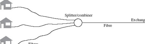
In the downstream direction – from the exchange to the home – multiplexed signals for all users are broadcast to all users, and the equipment in the home has to extract its ‘own’ signal. In the upstream direction there needs to be some mechanism for ensuring that the signals from each user do not interfere with each other, and the equipment at the exchange has to be able to extract and identify signals from each user. These are significant problems; trials of PONs have been run and the concept found to be technically feasible, but as with other FTTH experiments the economics are still in question.
One specific use of the PON concept is the Ethernet passive optical network (EPON) in the Ethernet in the first mile (EFM) standard being developed by the 802.3ah EFM Task Force of the IEEE 802 LAN/MAN standards committee.
4.5 Fibre in LANs
Fibre has been slower to be exploited in LANs than in the core transmission network, for similar reasons to the delay in the use of fibre in the access network, but as the data rate demanded of LANs has increased, the case for using fibre has strengthened.
Although Ethernet specifications (IEEE 802.3 series) have contained standards for the use of fibre backbones for some time, it was with the development of Gigabit Ethernet and 10 Gigabit Ethernet (10 GbE) standards that fibre became the main transmission medium. This section very briefly summarises the use of fibre in these two standards.
In this context 1300 nm is ‘long’ – because it is longer than 800 nm. In other contexts ‘long’ means wavelengths in the 1550 nm window in contrast to the ‘short’ 1300 nm window. And you have already met references to S-band, C-band and L-band, where ‘long’ means 1565–1625 nm and ‘short’ means 1460–1530 nm. It just goes to show that you have to be very careful with terms like long and short.
4.5.1 Gigabit Ethernet
Gigabit Ethernet specifies four categories:
1000BASE-SX, for transmission over multimode fibre using an LED in the 800 nm window (the wavelength is specified to be between 770 and 860 nm). The specification is for up to 275 m on 62.5/125 mm multimode fibre, or 550 m on 50/125 mm multimode fibre;
1000BASE-LX, for transmission over multimode or single-mode fibre using a laser in the 1300 nm window (specified to be between 1270 and 1355 nm). The distance on both 62.5/125 mm and 50/125 mm multimode fibre is specified as 550 m, and on single-mode fibre as 5 km;
1000BASE-CX specifies transmission on a shielded twisted-pair copper cable up to 25 m;
1000BASE-T specifies transmission on four pairs of unshielded twisted pairs up to 100 m.
In this context 1300 nm is ‘long’ - because it is longer than 800 nm. In other contexts ‘long’ means wavelengths in the 1550 nm window in contrast to the ‘short' 1300 nm window. And you have already met references to S-band, C-band and L-band, where ‘long’ means 1565-1625 nm and ‘short’ means 1460-1530 nm. It just goes to show that you have to be very careful with terms like long and short.
4.5.2 10 Gigabit Ethernet
The standard for 10 Gigabit Ethernet (IEEE 802.3ae, lOGbE) was approved in July 2002. The main use of lOGbE, initially at least, is for backbone networks which interconnect 10, 100 or 1000 Mbit/s Ethernet hubs. These hubs might be widely separated geographically, so the standard includes physical layer specifications specifically for WAN (wide area network) applications as well as LAN applications. The WAN specification is for operation at slightly under 10 Gbit/s, 9.95328 Gbit/s, so as to be compatible with the SDH.
SAQ 15
What level in the SDH hierarchy runs at 9.95328 Gbit/s?
Answer
9.95328 Gbit/s is the transmission rate of STM-64.
Both the WAN and LAN physical layers can use optical interfaces specified for use at 850 nm, 1310 nm and 1550 nm as follows (Figure 31):
10GBASE-S operates with a directly modulated 850 nm multimode laser diode and graded-index multimode fibre, at distances up to 300 metres;
10GBASE-L operates with a directly modulated 1310 nm single-mode laser diode and single-mode fibre, at distances up to 10 km;
10GBASE-E operates with an externally modulated 1550 nm single-mode laser diode and single-mode fibre, at distances up to 40 km.
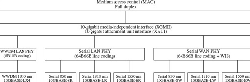
SAQ 16
If a 10GBASE-S interface used 50/125 mm fibre meeting the bandwidth-distance specification for Gigabit Ethernet of 500 MHz·km, approximately how far could the signal be transmitted? (The signalling rate of the 10GBASE-S interface is approximately 10.3 Gbaud.)
Answer
The minimum bandwidth that will allow a signalling rate of 10.3 Gbaud is:
The maximum transmission distance is therefore:
A target in the development of lOGbE was for a distance of at least 300 m on multimode fibre, and it is clear from the answer to SAQ 16 that this would not be possible with the 10GBASE-S interface on fibre that just meets the Gigabit Ethernet specification.
There are two solutions to this in 1 OGbE. One is to use new multimode fibre that has been developed with a higher specification, specifically for 1 OGbE. Referred to as ‘10 Gigabit Ethernet fibre’, this has a typical bandwidth-distance product of 2000 MHz·km.
Activity 18
What distance would be possible with this fibre?
Discussion
Repeating the calculation of SAQ 16 using the new specification leads to a distance of 2000/5150 = 388 m.
With this fibre the 300 m target can therefore be met (assuming that the power budget can also be balanced at 300 m).
The other solution is based on an additional interface specification, used only for the LAN physical layer (i.e. not the WAN physical layer), the 10GBASE-LX4 interface.
10GBASE-LX4 splits the data into four parallel streams and transmits them on four different wavelengths on a fibre. It therefore uses a type of WDM. The four wavelengths used are 1280 nm, 1300 nm, 1320 run and 1340 nm.
Activity 19
Into which of the ITU categories of WDM (CWDM, DWDM or WWDM) does this fit?
Discussion
The wavelength spacing (20 nm) makes it coarse wavelength division multiplexing, CWDM, although the actual wavelengths used are not those suggested in Recommendation G.694.2.
If you see reference to WWDM, make sure you know precisely what it means in context.
Unfortunately, although it most closely matches CWDM, the committee developing the IEEE 802.3ae standard chose to describe the scheme as wide wavelength division multiplexing, WWDM. The scheme most clearly does not fit with the ITU definition of WWDM.
10GBASE-LX4 can use either directly modulated multimode laser diodes or directly modulated single-mode laser diodes, and either multimode fibre (when it is specified to 300 m) or single-mode fibre (when it is specified to 10 km).
On multimode fibre it is capable of 300 m on existing (Gigabit Ethernet compliant) fibre.
4.6 Conclusion to Section 4
This brief account has introduced a few of the most rapidly developing areas of optical-fibre communications as of January 2004. By the time you are reading it things will certainly have moved on, and if you want to find the current state of the art you should read journals such as IEEE Communications Magazine or trade magazines such as Lightwave. It is also possible to find out more on the world wide web.
I hope you will agree that this is a fascinating field, and that you will be encouraged to study it further.
Conclusion
The building blocks of a basic optical-fibre communications link are the modulated light source, the fibre and the detector. There are choices to be made between different types of light source and fibre, with trade-offs between cost and performance. For example, for high signalling rates over long distances single-mode fibre will be used with a single-mode laser (possibly with external modulation) operating in the 1550 nm window, whereas for short-distance links operating at lower signalling rates multimode fibre will be used with a directly modulated LED operating at around 850 nm.
The maximum transmission distance without regeneration at a given signalling rate over an optical-fibre link is limited by either attenuation or inter-symbol interference. The effects of attenuation are determined by calculating the power budget for the link. The main cause of inter-symbol interference in multimode fibre is multimode distortion, which is characterised by the bandwidth-distance product of the fibre. Causes of inter-symbol interference in single-mode fibre include dispersion and polarization mode distortion.
Optical amplifiers can overcome the limits due to attenuation, and the effects of dispersion can be mitigated by using dispersion-shifted fibre or through the use of dispersion compensation. Increasing the capacity of a fibre through increased signalling rates becomes more difficult as the signalling rates rise above 40 Gbaud, however, and the alternative of using wavelength division multiplexing (WDM) is preferable.
WDM is usually done in the 1550 nm window because erbium-doped fibre amplifiers can then be used to amplify all channels simultaneously. Fibre non-linearities become important when dense WDM is used, leading to the need for non-zero dispersion-shifted fibre.
Beyond the simple point-to-point link, devices such as fibre splitters and combiners, WDM devices and optical switches allow more sophisticated use of optical-fibre communication, leading ultimately to the concept of an all-optical network.
Appendices
Appendix 1 Terminology
After studying this unit you should be able to explain the meaning of the following terms:
all-optical network
angle-polished convex connector
bandwidth-distance product
chirp
combiner
connector
continuous wave operation
dense wavelength division multiplexing
direct modulation directional coupler dispersion
dispersion compensation dispersion-shifted fibre electro-optic material excess loss external modulation extinction ratio four-wave mixing Fresnel reflection graded-index fibre index-matching fluid (or gel) insertion loss laser diode
light-emitting diode
lithium niobate
micro-electro-mechanical system
multimode distortion
non-zero dispersion-shifted fibre
photodiode
physical contact connector
polarization mode
polarization mode distortion
power budget
Raman amplifier
receive sensitivity
refractive index
return loss
semiconductor optical amplifier
single-mode laser diode
splice
splitter
star coupler
step-index fibre
stimulated Raman scattering
total internal reflection
tuneable laser
Appendix 2 Acronyms
| APC | angle-polished convex (connector) |
| ASE | amplified spontaneous emission |
| ASK | amplitude shift keying |
| cw | continuous wave |
| DSF | dispersion-shifted fibre |
| DWDM | dense wavelength division multiplexing |
| EDFA | erbium-doped fibre amplifier |
| FWM | four-wave mixing |
| IEC | International Electrotechnical Commission |
| IEE | Institution of Electrical Engineers (UK) |
| IEEE | Institute of Electrical and Electronics Engineers (USA) |
| ISI | inter-symbol interference |
| ITU-T | International Telecommunication Union – Telecommunication Standardization Sector |
| LAN | local area network |
| LED | light-emitting diode |
| MEMS | micro-electro-mechanical system |
| NZ-DSF | non-zero dispersion-shifted fibre |
| OOK | on-off keying |
| PC | physical contact (connector) |
| PMD | polarization mode distortion |
| RIN | relative noise intensity |
| SBS | stimulated Brillouin scattering |
| SLA | semiconductor laser amplifier |
| SOA | semiconductor optical amplifier |
| SPM | self-phase modulation |
| SRS | stimulated Raman scattering |
| WDM | wavelength division multiplexing |
| XPM | cross-phase modulation |
References
Acknowledgements
Except for third party materials and otherwise stated (see terms and conditions), this content is made available under a Creative Commons Attribution-NonCommercial-ShareAlike 4.0 Licence
Course image: Kohei314 in Flickr made available under Creative Commons Attribution-NonCommercial-ShareAlike 2.0 Licence.
Grateful acknowledgement is made to the following source for permission to reproduce material within this unit:
Table 5: 'Nominal central wavelengths for CWDM’, ITU-T G.694.2 Prepublished Recommendation: Spectral Grids for WDM Applications: CWDM wavelength grid, International Telecommunication Union;
Table 6: 'Nominal central frequencies of the DWDM grid’, ITU-T G.691.1 Prepublished Recommendation: Spectral Grids for WDM Applications: DWDM frequency grid, International Telecommunication Union.
All other written material contained within this unit originated at the Open University
Don't miss out:
If reading this text has inspired you to learn more, you may be interested in joining the millions of people who discover our free learning resources and qualifications by visiting The Open University - www.open.edu/ openlearn/ free-courses