Surfaces
Use 'Print preview' to check the number of pages and printer settings.
Print functionality varies between browsers.
Printable page generated Thursday, 25 April 2024, 6:32 PM
Surfaces
Introduction
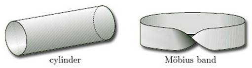
This course is concerned with a special class of topological spaces called surfaces. Common examples of surfaces are the sphere and the cylinder; less common, though probably still familiar, are the torus and the Möbius band. Other surfaces, such as the projective plane and the Klein bottle, may be unfamiliar, but they crop up in many places in mathematics. Our aim is to classify surfaces – that is, to produce criteria that allow us to determine whether two given surfaces are homeomorphic.
This OpenLearn course provides a sample of Level 3 study in Mathematics
Learning outcomes
After studying this course, you should be able to:
explain the terms surface, surface in space, disc-like neighbourhood and half-disc-like neighbourhood
explain the terms n-fold torus, torus with n holes, Möbius band and Klein bottle
explain what is meant by the boundary of a surface, and determine the boundary number of a given surface with boundary
construct certain compact surfaces from a polygon by identifying edges
explain how a surface in space can be regarded as a topological space.
1 Topological spaces and homeomorphism
Two topological spaces (X, TX) and (Y, TY) are homeomorphic if there is a bijection f : X → Y that is continuous, and whose inverse f−1 is also continuous, with respect to the given topologies; such a function f is called a homeomorphism. The relation ‘is homeomorphic to’ between topological spaces is the most fundamental relation in topology, because two topological spaces that are homeomorphic are indistinguishable from a topological point of view – they are topologically equivalent. An alternative definition of a homeomorphism is that a bijection f : X → Y is a homeomorphism if and only if both f and f−1 map open sets to open sets. Thus, if (X, TX) and (Y, TY) are homeomorphic, then not only are the elements of X and Y in one–one correspondence, but so also are their open sets. We can thus regard (Y, TY) as being essentially the same space as (X, TX), so far as its purely topological properties are concerned: (X, TX) and (Y, TY) are merely two different ways of presenting the same space.
It is therefore useful to be able to determine whether two given topological spaces are homeomorphic. Of course, if we can find a specific homeomorphism between them then the question is answered; but if we fail to find a homeomorphism then we cannot deduce that there isn't one. So looking for a particular homeomorphism may not be the best approach. What we want are criteria that enable us to tell whether two given surfaces are homeomorphic without our having to try to construct a specific homeomorphism between them.
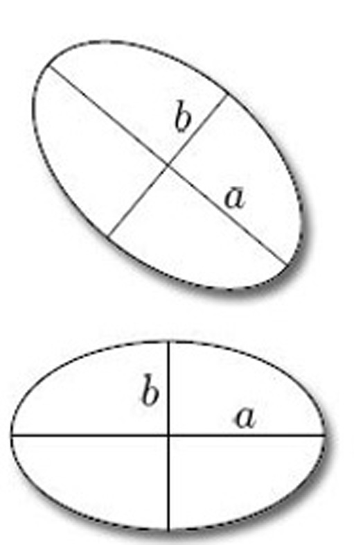
A similar situation, which may help to clarify what is involved, is the following. A map between metric spaces that preserves distances is called an isometry, and two subsets of a metric space that are related by an isometry are essentially the same, so far as their metrical properties are concerned. For example, consider the collection of ellipses in ![]() 2, with the Euclidean metric. Two ellipses are isometric if and only if the lengths of their major axes are the same, and the lengths of their minor axes are the same (see Figure 1). These two criteria enable us to determine whether two given ellipses are isometric without our having to construct a specific isometry between them: we simply compare the lengths of their axes. We say that the lengths of the major and minor axes classify ellipses in
2, with the Euclidean metric. Two ellipses are isometric if and only if the lengths of their major axes are the same, and the lengths of their minor axes are the same (see Figure 1). These two criteria enable us to determine whether two given ellipses are isometric without our having to construct a specific isometry between them: we simply compare the lengths of their axes. We say that the lengths of the major and minor axes classify ellipses in ![]() 2up to isometry.
2up to isometry.
Notice that, in the phrase ‘classify ellipses in ![]() 2 up to isometry’, we have specified the class of figures under consideration (ellipses in
2 up to isometry’, we have specified the class of figures under consideration (ellipses in ![]() 2): our criteria apply only to these particular figures in the plane, and we make no claim that other figures can be classified up to isometry in a similar way. Note also the importance of including the qualification ‘up to isometry’, since all ellipses are homeomorphic.
2): our criteria apply only to these particular figures in the plane, and we make no claim that other figures can be classified up to isometry in a similar way. Note also the importance of including the qualification ‘up to isometry’, since all ellipses are homeomorphic.
In this course, our main task is to define a certain class of surfaces called compact surfaces, and then to specify criteria that allow us to determine whether two given compact surfaces are homeomorphic. These surfaces can be classified using just three criteria, as we shall show. Indeed, just as we can classify ellipses in ![]() 2 up to isometry by specifying just two numbers (the lengths of the major and minor axes), so we can classify all compact surfaces up to homeomorphism by specifying just three numbers. The appropriate theorem – the Classification Theorem – is stated later in this course. Before we state the Classification Theorem, we give examples of surfaces, show how they can be manipulated, defined and represented, and examine some of their important properties.
2 up to isometry by specifying just two numbers (the lengths of the major and minor axes), so we can classify all compact surfaces up to homeomorphism by specifying just three numbers. The appropriate theorem – the Classification Theorem – is stated later in this course. Before we state the Classification Theorem, we give examples of surfaces, show how they can be manipulated, defined and represented, and examine some of their important properties.
The spirit in which we explore surfaces in this course arises from the way that the theory of surfaces relates to the rest of topology, and that in turn is reflected in the history of these subjects. When studying surfaces we can proceed a long way with intuitive concepts, and the subject is often studied in that fashion. Today we may appeal to these intuitions, secure in the knowledge that the intuitively appealing theorems can be proved rigorously. Indeed, the precise definitions and rigorous proofs appearing in the literature frequently involve subtle and difficult arguments of a kind otherwise out of keeping with geometric topology, and may add little to our understanding of the underlying concepts.
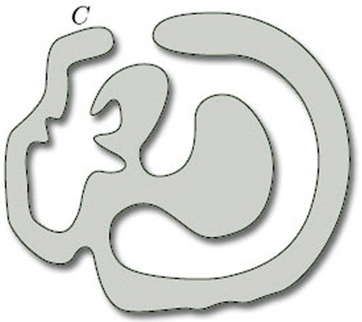
An example is the so-called Jordan Curve Theorem, which asserts that any curve in the plane that is homeomorphic to a circle divides the plane into two regions, one bounded (the ‘inside’ of the curve) and the other unbounded (the ‘outside’); Figure 2 shows such a curve C in the plane, with its inside shaded. Although the statement of the Jordan Curve Theorem is entirely plausible – indeed, it is fundamental to many parts of mathematics – the theorem is difficult to prove. In fact, it is likely that few mathematicians have ever seen a proof, because such proofs merely confirm what we already believe. It is good to have a proof, of course, but we do not consider it essential to prove all of the results in this course. Examining the proof of the Jordan Curve Theorem reveals no particularly counter-intuitive complications, and so we omit the proof.
In this course we indicate when concepts are to be understood at an intuitive level, and when more precise definitions, theorems and proofs are required. Where possible, we provide rigorous definitions and proofs.
2 Examples of surfaces
2.1 Surfaces in space
In Section 2 we start by introducing surfaces informally, considering several familiar examples such as the sphere, cube and Möbius band. We also illustrate how surfaces can be constructed from a polygon by identifying edges. A more formal approach to surfaces is presented at the end of the section.
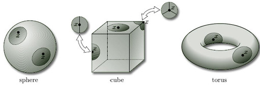
Figure 3 shows some simple examples of surfaces in three-dimensional space.
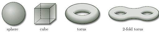
Since we are interested only in the surface of such objects, rather than the interior, you should always think of such objects as being hollow, rather than solid. Such surfaces, being subsets of ![]() 3, are given the subspace topology from
3, are given the subspace topology from ![]() 3.
3.
In each of the examples in Figure 3, the surface is locally like part of the plane, as illustrated in Figure 4. This means that, for each point x of the surface, we can find a subset of the surface that contains x and is homeomorphic to an open disc in the plane: we call such a subset a disc-like neighbourhood of x. (A neighbourhood of a point x is an open set containing x.) Such a neighbourhood is an open subset of the surface in the subspace topology that it inherits from ![]() 3.
3.
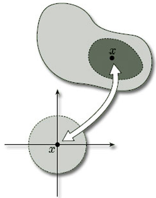
Figure 5 shows some disc-like neighbourhoods in three of the surfaces of Figure 3. Notice that a disc-like neighbourhood may be curved or bent in space, or may even have folds in it.
Problem 1
Draw some disc-like neighbourhoods on a 2-fold torus.
Answer
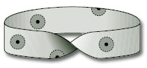
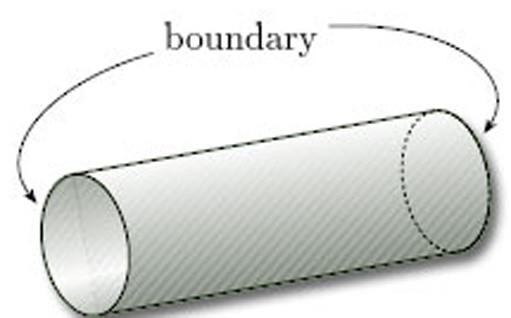
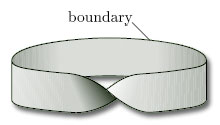
All the objects we wish to consider as surfaces have many points with disc-like neighbourhoods. However, there are some surfaces where some of the points do not have such neighbourhoods. Two common examples are shown in Figure 6 – a hollow cylinder, open at both ends, and a Möbius band.
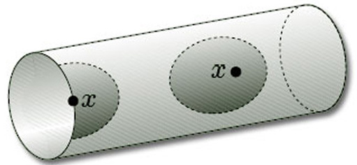
Two neighbourhoods of points on the cylinder are shown in Figure 7. These illustrate that, except for the points at the ends of the cylinder, each point has a disc-like neighbourhood; but the points at the ends have no such neighbourhoods. Instead, each such endpoint x has a half-disc-like neighbourhood – a subset that is homeomorphic to an open half-disc in the upper half-plane, considered as a subspace of ![]() 2, as shown in Figure 8. Such a neighbourhood is again an open subset of the surface in the subset topology that it inherits from
2, as shown in Figure 8. Such a neighbourhood is again an open subset of the surface in the subset topology that it inherits from ![]() 3.
3.
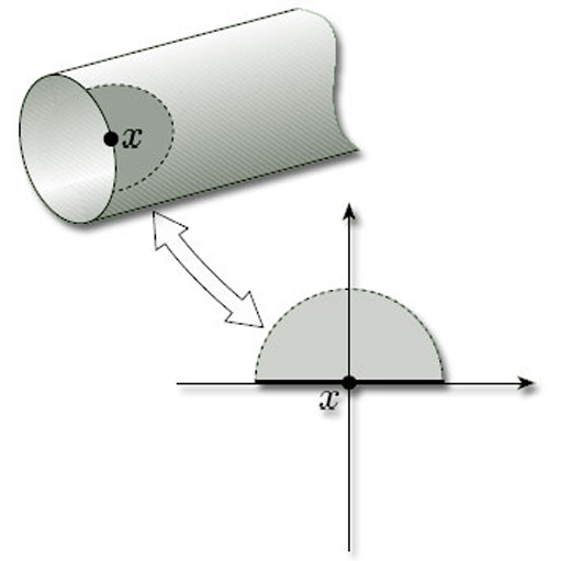
The upper half-plane includes the points on the horizontal axis. The open half-discs are those with diameter along that axis and include the axis points; they are open subsets of the closed half-plane in the subspace topology inherited from ![]() 2.
2.
Problem 2
Draw some disc-like and half-disc-like neighbourhoods on a Möbius band.
Answer
In fact, all the objects we wish to consider have surfaces that are characterised as consisting of points that have either disc-like or half-disc-like neighbourhoods. This leads to the following provisional definition.
Provisional definition
A surface is a topological space (X, T) with the property that each point of X has a neighbourhood that is homeomorphic either to an open disc in the plane or to an open half-disc in the upper half-plane, i.e. given any point x ![]() X, there is an open set U containing x such that U is homeomorphic either to an open disc in
X, there is an open set U containing x such that U is homeomorphic either to an open disc in ![]() 2 or to an open half-disc in the upper half-plane with the subspace topology inherited from the Euclidean topology on
2 or to an open half-disc in the upper half-plane with the subspace topology inherited from the Euclidean topology on ![]() 2. The open set U is called a disc-like neighbourhood, or half-disc-like neighbourhood of x, as the case may be.
2. The open set U is called a disc-like neighbourhood, or half-disc-like neighbourhood of x, as the case may be.
(We shall modify this definition slightly at the end of this section.)
This idea of points of a surface having disc-like neighbourhoods or half-disc-like neighbourhoods is crucial to the concept of a surface. In the following worked problem we present an object that looks as though it might be a surface, but fails to be so because it has a point with no such neighbourhood.
Worked problem 1
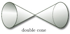
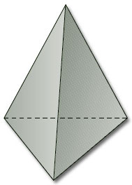
Explain why the double cone, open at both ends, is not a surface.
Solution
Although most points on the double cone have disc-like or half-disc-like neighbourhoods, the point z in the middle, indicated in Figure 10(a), does not. One way to see this is to note that if we remove the point z, then the neighbourhood breaks into two pieces, as shown in Figure 10(b). This cannot be the case if the neighbourhood is homeomorphic to a disc or half-disc: removing a single point from a disc or half-disc cannot split it into two pieces.
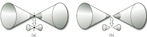
Since we have found a point with no disc-like or half-disc-like neighbourhood, the double cone is not a surface.
Problem 3
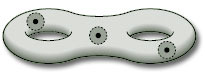
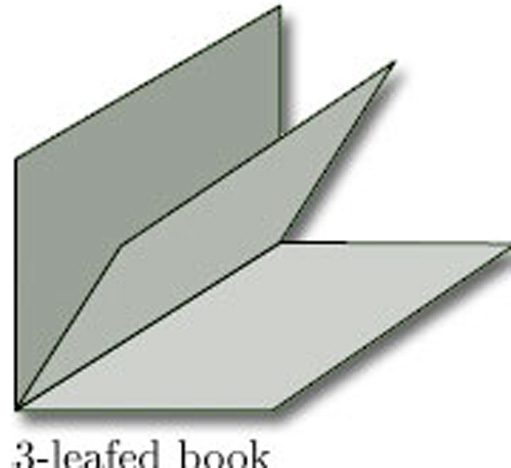
Explain why the 3-leafed book, illustrated in Figure 11, is not a surface.
Answer
No point on the spine of a 3-leafed book has a disc-like or half-disc-like neighbourhood. If we remove the spine, then the neighbourhood of any point on the spine breaks into three pieces, as shown. This cannot be the case if the neighbourhood is homeomorphic to a disc or half-disc.
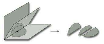
Since no point on the spine has a disc-like or half-disc-like neighbourhood, the 3-leafed book is not a surface.
The points of a surface with half-disc-like neighbourhoods, such as the endpoints of a cylinder, can be thought of as lying on the boundary of the surface.
Definitions
Let S = (X, T) be a surface.
A boundary point of S is a point of X for which every neighbourhood contains a half-disc-like neighbourhood.
The boundary of S is the set of all boundary points of S.
A surface with boundary is a surface whose boundary is non-empty.
A surface without boundary is a surface with no boundary points.
An example of a surface with boundary is a cylinder, whose boundary consists of the two circular ends (Figure 12). An example of a surface without boundary is a sphere, since each point has a disc-like neighbourhood (Figure 5).
Problem 4
Identify the boundary of each of the following surfaces:
(a) a Möbius band;
(b) a torus.
Answer
(a) The boundary consists of the single edge.
(b) Since each point has a disc-like neighbourhood, there is no boundary, i.e. the boundary is the empty set.
The following theorem describes the boundary of a surface.
Theorem 1
The boundary of a surface is composed of a finite number of arcs, each of which is homeomorphic to a circle or to a unit interval, or it is the empty set.
(We omit the proof, which is beyond the scope of this course.)
Up to now our surfaces have been ones that can be embedded in three-dimensional space. We give these a special name.
Provisional definition
A surface in space is a surface (X, TX) where X is a subset of ![]() 3 and TX is the subspace topology on X inherited from the Euclidean topology T on
3 and TX is the subspace topology on X inherited from the Euclidean topology T on ![]() 3.
3.
Since our definition of a surface is provisional, this definition of a surface in space is provisional also.
In Section 2.3 we shall meet some surfaces that cannot be embedded in three-dimensional space.
2.2 Surfaces in space
In this section we present a wide range of examples of surfaces in space.
2.2.1 Surfaces without boundary
Examples of surfaces without boundary are a sphere and a torus. Other examples are the following:
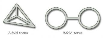
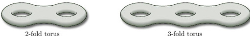
n-fold toruses
Figure 13 depicts a 2-fold torus and a 3-fold torus, with two and three rings respectively. An n-fold torus, for any positive integer n has n rings. (A 1-fold torus is simply a torus, as in Figure 3.)
Toruses do not have to be considered as ‘n-ringed doughnuts’ as in Figure 13; they can also usefully be described as ‘spheres with n handles’, as Figure 14 illustrates.
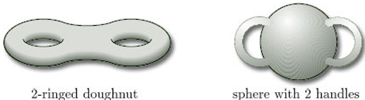
In fact, any homeomorphic representation will do, as we shall see in Section 2.4.
2.2.2 Hollow tubing surfaces
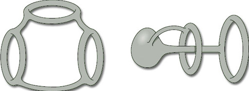
In their doughnut-shaped representation, toruses can be thought of as being hollow tubes. Many other surfaces in space can also be drawn as if they were made of hollow tubing. Figure 15 shows two such examples.
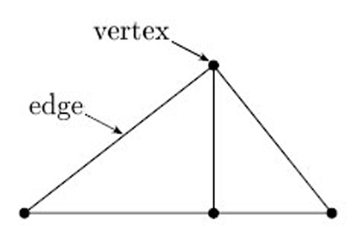
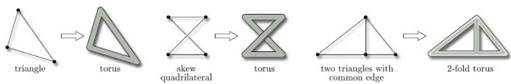
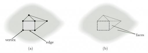
There is an easy way of constructing hollow tubing surfaces. Start with a finite set of points in three-dimensional space, called vertices, and connect them together by a finite set of lines, called edges, that meet only at the vertices, as shown in Figure 16: such a configuration is called a connected graph. We then obtain a surface by ‘thickening each edge’ of the connected graph into a hollow tube, as illustrated in Figure 17: the resulting surface, called a thickened graph, can be thought of as a hollow tube wrapping the original connected graph.
Problem 5
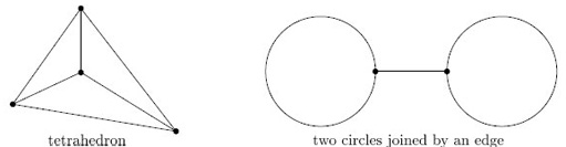
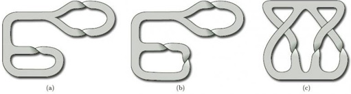
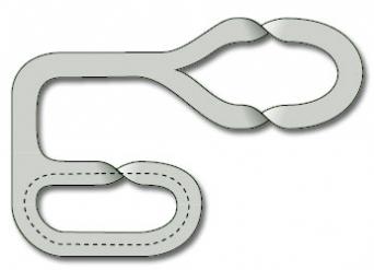
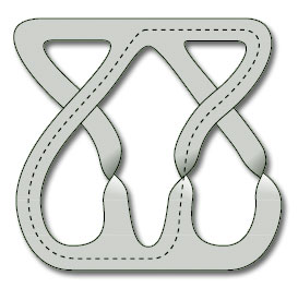
For each of the connected graphs in Figure 18, draw the associated thickened graph.
Answer
2.2.3 Surfaces with boundary
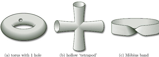
Examples of surfaces with boundary are a cylinder and a Möbius band. Other examples are the following:
Surfaces with holes
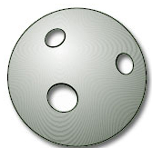
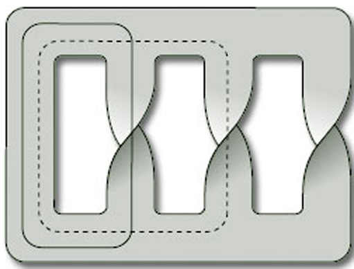
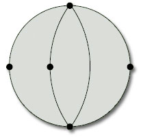
We can obtain a surface with boundary by taking any surface without boundary and punching some holes in it by removing open discs. For example, Figure 19 shows a sphere with 3 holes. The boundary of the surface with holes consists of the boundaries of the holes.
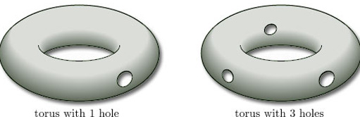
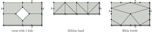
Another example is a torus with holes. Figure 20 illustrates a torus with 1 hole and a torus with 3 holes. We can have a torus with k holes for any positive integer k. (Do not confuse a torus with k holes and a k-fold torus.)
We can also combine the notions of an n-fold torus and a torus with k holes to draw an n-fold torus with k holes, for any positive integers n and k. For example, Figure 21 depicts a 2-fold torus with 4 holes.
Problem 6
Draw a 4-fold torus with 5 holes and a 5-fold torus with 4 holes. What is the boundary of each surface?
Answer
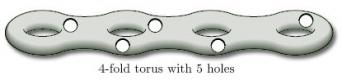
The boundary consists of the boundaries of the 5 holes.
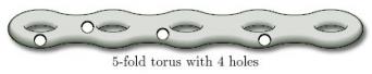
The boundary consists of the boundaries of the 4 holes.
Paper surfaces
Other surfaces can be drawn as if they were made from thin strips of material, such as paper. The surface consists of one side of the paper only. Two such surfaces are shown in Figure 22. Notice how some parts of a surface can cross over, or under, other parts.
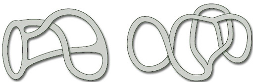
2.2.4 Boundary numbers
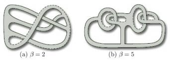
In a surface with boundary, the boundary may consist of more than one piece. For example, the boundary of a cylinder, or of a torus with two holes, consists of two pieces, as shown in Figure 23.
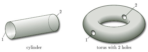
The separate pieces forming the boundary of a surface S are called the boundary components of S. The number of boundary components is the boundary number of S, denoted by β. Thus β = 2 for each of the surfaces in Figure 23.
For a surface without boundary, there are no boundary components, so β = 0.
(β is the Greek letter beta.)
To find the boundary numbers of paper surfaces, it is convenient to use coloured pens to trace around the boundary. Doing this, we find that the two boundary numbers of the surfaces in Figure 22 are β = 4 and β = 3, as shown in Figure 25.
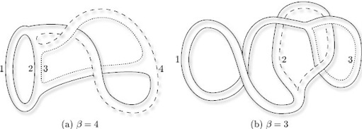
Problem 8
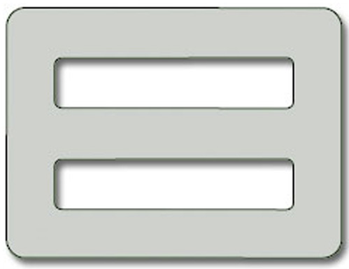
Find the boundary number β of each of the paper surfaces in Figure 26.
Answer
The boundary number β is one of the three characteristic numbers that we use to classify compact surfaces.
2.3 Paper-and-glue constructions
In this section we show how to construct surfaces by taking a piece of paper in the shape of a polygon and gluing some of its edges together. The surfaces that we obtain occupy a central position in this course, as you will see.
2.3.1 Cylinder
The simplest example of a paper-and-glue construction is to make a rectangle into a cylinder by gluing together two opposite edges. We take a closed rectangle ABB' A' in the plane and identify the opposite edges AB and A'B', as shown in Figure 27. This means that:
-
we imagine A and A' to be the same point (which we'll label A);
-
we imagine B and B' to be the same point (which we'll label B);
-
we match up all corresponding pairs of points in between (such as P and P') as shown.
The direction of the identification is given by the order of the letters labelling an edge: labelling an edge AB implies a direction from A to B; similarly A'B' implies a direction from A' to B'.
Note that we have drawn arrowheads on the edges AB and A'B' of the rectangle to emphasise that they are to be identified in the same direction.
We also obtain a cylinder if we identify the edges AA' and BB'.

2.3.2 Möbius band
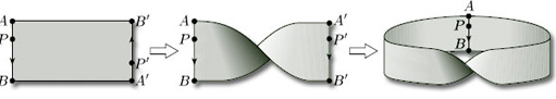
Let us now see what happens if we try to identify two opposite edges of a rectangle in opposing directions. (Here, we are identifying the two ends of the rectangle rather than the top and bottom.) We start with a rectangle, as before, but this time the edges to be identified have their arrowheads pointing in opposite directions. This means that we cannot glue the edges directly, but have to twist one of them through ![]() radians before gluing. More formally, we take a closed rectangle ABA'B' in the plane and identify the opposite edges AB and A'B', as shown in Figure 28. This means that:
radians before gluing. More formally, we take a closed rectangle ABA'B' in the plane and identify the opposite edges AB and A'B', as shown in Figure 28. This means that:
- we imagine A and A' to be the same point;
- we imagine B and B' to be the same point;
- we pair up all corresponding points in between (such as P and P'), taking note of the directions of the arrowheads.
We obtain a Möbius band.
Again, the labelling AB implies a direction from A to B, and similarly A'B' implies a direction from A' to B'.
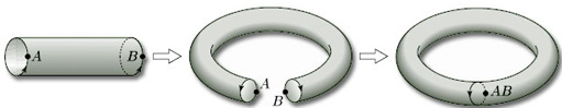
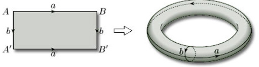
2.3.3 Torus
Let us now return to the cylinder we obtained in Figure 27. What happens if we bend it around and glue the two ends? Now, continuing with our idea of identifying edges of our original rectangle, we want to bend the cylinder round and glue its ends in such a way that the points A and B are identified. Furthermore, bending as shown in Figure 29 corresponds to identifying the edges AA' and BB' of the original rectangle in the same direction, as indicated in the figure. We obtain a torus.
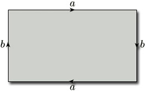
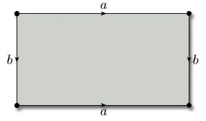
In terms of our original rectangle, the whole construction process corresponds to identifying opposite edges in pairs in the directions indicated by the arrowheads in Figure 30. For ease of reference, we label each pair of edges that is to be identified with the same letter, a for the first pair to be identified and b for the second pair.
We often omit the vertex labels from polygons used to construct surfaces by identification and simply use these edge labels.
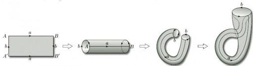
2.3.4 Klein bottle
There are two other surfaces that can be obtained by identifying both pairs of opposite edges of a rectangle. In one of these, shown in Figure 31, we first identify the edges AB and A'B', labelled a, in the direction shown by the arrowheads. This gives us a cylinder, as before. We then try to identify the cylinder ends, labelled b, in opposite directions, as indicated by the arrowheads – this is equivalent to identifying the edges A'A and BB', labelled b, of the original rectangle. Unfortunately, this cannot be done in three dimensions, and so is hard to visualise: if we try to link the ends, the cylinder has to ‘pass through itself’. So, although we have a surface, it is not a surface in space. It is called a Klein bottle.
2.3.5 Projective plane
The final surface that can be obtained by identifying edges of a rectangle is even more complicated. Again it cannot be constructed in three dimensions, so is not a surface in space and is hard to visualise. This time we identify both pairs of opposite edges of the rectangle in opposite directions, as indicated by the arrowheads in Figure 32: we identify the edges AB and B'A' (labelled a) and the edges A'A and BB' (labelled b). The resulting surface is called the projective plane.
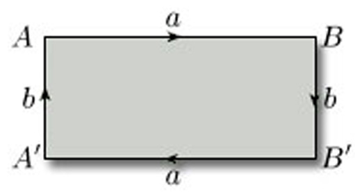
The existence of the Klein bottle and the projective plane, which are not surfaces in space, is one reason why mathematicians cannot restrict their study of surfaces to surfaces in space.
We discuss the projective plane in Section 3.
2.3.6 Torus with 1 hole
We need not restrict ourselves to rectangles: we can also build surfaces by identifying edges of other polygons. For example, if we start with a pentagon and identify two pairs of its edges as shown in Figure 33, what do we get? Identifying the edges labelled a and c in the directions indicated, we obtain a cylinder with a hole; the boundary of the hole is the edge labelled c. If we now identify the edges labelled b (now at each end of the cylinder) in the directions indicated, after some bending and stretching we obtain a torus with a hole.
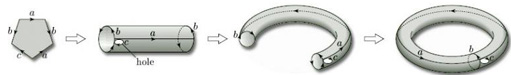
From now on, we shall usually put a direction on every edge (such as edge c), even if it is not to be identified. For such an edge, we can choose an arbitrary direction.
2.3.7 Two-fold torus
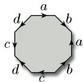
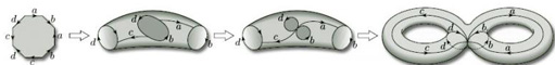
As the polygons become more complicated, so the identifications become more difficult to visualise. For example, what happens if we try to identify the edges of an octagon in pairs, as indicated by the edge labels and arrowheads in Figure 34? Figure 35 shows that identifying, in the directions indicated, the edges labelled a and the edges labelled c results, after some bending and stretching, in a cylinder bounded by edges labelled b and d. If we now identify, in the directions indicated, the edges labelled b and the edges labelled d, we obtain, after some bending and stretching, a 2-fold torus. One way of seeing this is first to pull together the edges labelled a and c in the holed cylinder, creating two holes bounded by edges b and d, and then to bend round the cylinder ends to meet these holes.
In a similar way, one could obtain a 3-fold torus by identifying the twelve edges of a dodecagon in pairs, and in general an n-fold torus from a 4n-sided polygon, for all natural numbers n.
2.3.8 Sphere
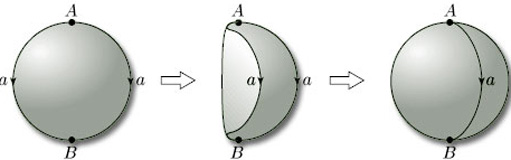
Surfaces can be constructed in a similar way from plane figures other than polygons. For example, starting with a disc, we can fold the left-hand half over onto the right-hand half, and identify the edges labelled a, as shown in Figure 36; this is rather like zipping up a purse, or ‘crimping’ a Cornish pastie. We can then stretch and inflate the object so obtained until we obtain a sphere.
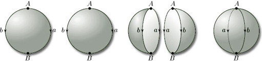
We can even start with more than one plane figure. For example, a sphere can be formed from two discs by identifying edges as shown in Figure 37 and then inflating.
Problem 9
Which surfaces are obtained by identifying edges (in the given directions) in each of the triangles in Figure 38?
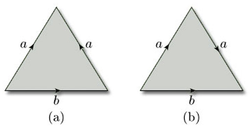
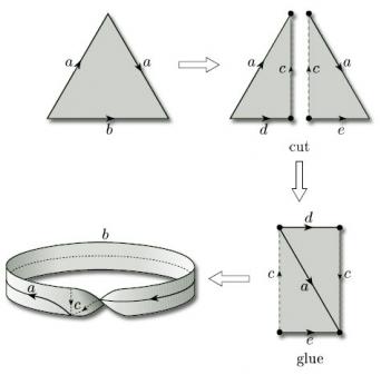
Hint: In (b), you might consider cutting the triangle before identifying the edges, and then repairing the cut.
Answer
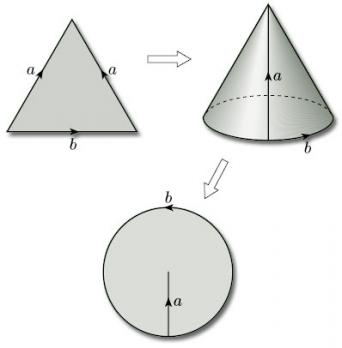
(a) Identifying the edges we obtain a cone which can then be flattened out. The result is a disc.
(b) The three vertices of the triangle are all identified to a single point which lies on the boundary of the resulting surface; the two edges that are identified become a single closed curve through this point. The result is a Möbius band. One way of seeing this is to bisect the triangle, glue the two parts together by identifying the edges labelled a, to create a rectangle, then repair the bisection (which needs a twist).
Throughout this section, our emphasis has been on describing the edge identifications geometrically. A more rigorous treatment, involving the so-called ‘identification topology’, is given in Section 5.
2.4 Homeomorphic surfaces
As we stated in Section 1, our aim is to classify surfaces up to homeomorphism. So it is worthwhile spending a little time examining what sorts of transformations of surfaces are homeomorphisms. We shall restrict the description to surfaces in space, as these are easier to deal with, though the result at the end of this subsection applies to all surfaces.
Recall that a homeomorphism between two topological spaces (such as surfaces in space) is a bijection with the property that both f and its inverse f−1 preserve open sets.
Roughly speaking, homeomorphisms between surfaces in space are of two kinds. One kind includes any transformation of a surface in space that can be achieved by bending, stretching, squeezing or shrinking the surface. These maps are certainly one–one and onto, and (intuitively, at least) seem to be continuous – and thus are bijections. They would also seem to preserve open sets, if we remember that the topology of a surface in space is the subspace topology inherited from ![]() 3. So, essentially, we can achieve a homeomorphism by treating a surface in space as if it were made from a sheet of rubber and then bending, stretching, squeezing or shrinking it. Topology is sometimes called rubber-sheet geometry.
3. So, essentially, we can achieve a homeomorphism by treating a surface in space as if it were made from a sheet of rubber and then bending, stretching, squeezing or shrinking it. Topology is sometimes called rubber-sheet geometry.
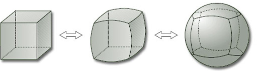
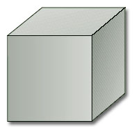
For example, the sphere in its usual round form and in various lumpy forms (such as a cube) are homeomorphic, as we can see by pumping air into the lumpy one and inflating it as if it were a balloon, as illustrated in Figure 39. If the surface has sharp edges and vertices, then stretching and smoothing it can remove these edges and vertices.
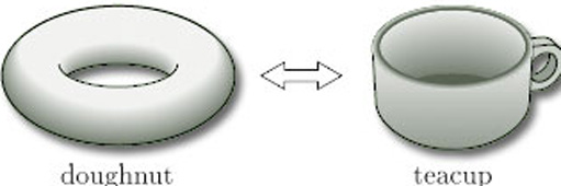
This sort of homeomorphism also explains why we are able to draw n-fold toruses either in doughnut form or in the form of a sphere with handles – both representations are topologically equivalent. It also explains the description of a topologist as someone who doesn't know the difference between a doughnut and a teacup, since both shapes are topologically equivalent under a homeomorphism of this kind (Figure 40).
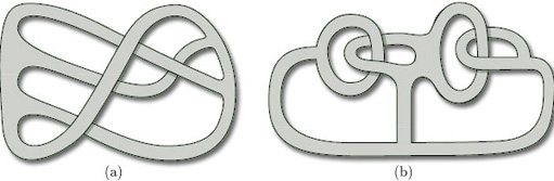
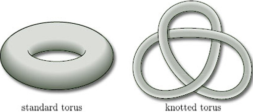
As an example of the other kind of homeomorphism, consider the torus in its usual form, sometimes referred to as its standard form, and in a knotted form, as shown in Figure 41.
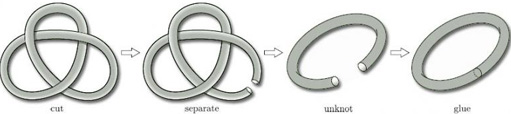
It is impossible to ‘unknot’ the knotted torus just by bending, stretching, squeezing or shrinking it – but we can cut it and open it out, rearrange it as a cut torus, and then glue it back together, as shown in Figure 42.
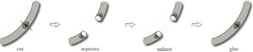
Provided that we are able to join the points on either side of the cut exactly as they were beforehand, the whole operation defines a homeomorphism between the two surfaces. If this seems surprising, look at the neighbourhood of a point on the cut, as enlarged in Figure 43: clearly, open discs are mapped to open discs without any change.
To sum up, two surfaces in space are homeomorphic if we can bend, stretch, squeeze or shrink one into the other and/or if we can cut one and then, after some bending, stretching, squeezing or shrinking, glue it back together (making sure to join the points on either side of the cut exactly as beforehand) to form the other. We thus have a practical and intuitive way of demonstrating that surfaces in space are homeomorphic.
There are also practical ways of showing that two surfaces in space are not homeomorphic. One is to consider the boundary number of the surface.
Theorem 2
Two surfaces that are homeomorphic have the same boundary number.
(We omit the proof, which is beyond the scope of this course.)
2.4.1 Remarks
-
This theorem applies to all surfaces and not just to surfaces in space.
-
This theorem tells us that the boundary number is a topological invariant for surfaces, i.e. a property that is invariant under homeomorphisms.
-
It follows from the theorem that two surfaces with different boundary numbers cannot be homeomorphic. It does not follow that two surfaces with the same boundary number are homeomorphic – for example, a sphere and a torus both have boundary number 0, but are not homeomorphic (as we demonstrate below).
-
Another consequence of the theorem is that a surface with non-zero boundary number cannot be homeomorphic to a surface with boundary number 0 – that is:a surface with boundary cannot be homeomorphic to a surface without boundary.
This seems reasonable, because such a homeomorphism would have to take the half-disc-like neighbourhoods of a boundary point to disc-like neighbourhoods of the image point.
Problem 10
Use boundary numbers to show that a Möbius band and a 2-fold torus are not homeomorphic.
Answer
For the Möbius band, β = 1; for the 2-fold torus, β = 0. Since these numbers are different, the surfaces are not homeomorphic, by Theorem 2.
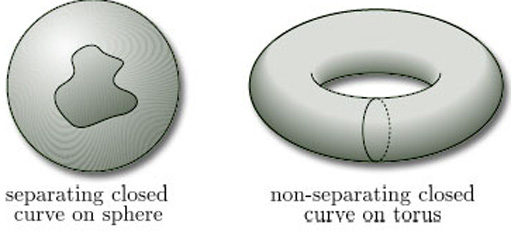
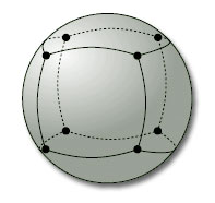
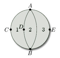
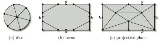
For surfaces in space with the same boundary number, there is another practical test that can sometimes be used to confirm that they are not homeomorphic. It requires the consideration of closed curves on the surface. For example, consider a sphere and a torus, both of which have boundary number 0. Observe that any closed curve on the sphere that does not cross itself separates the sphere into two regions, whereas there are closed curves on the torus that do not (see Figure 44). If the sphere and the torus were homeomorphic, then a non-separating curve on the torus would map by the homeomorphism onto a non-separating curve on the sphere, which is not possible. (This is the Jordan Curve Theorem mentioned in Section 1.)
2.5 Defining surfaces
In Section 2.1 we gave a provisional definition of a surface. The aim of this section is to formalise that definition. To do that, we need to specify three further requirements of a candidate topological space, beyond those given in the provisional definition.
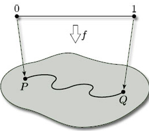
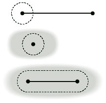
The first requirement is that the surface should be in ‘just one piece’. We can ensure this by requiring the surface to be path-connected: this means that any two points P and Q on the surface can be joined by a curve that lies entirely in the surface. In mathematical terms, this means that there is a continuous map f from the interval [0, 1] to the surface, such that f(0) = P and f(1) = Q (see Figure 45).
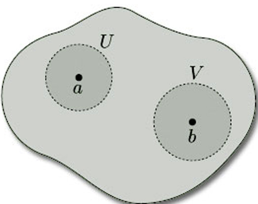
The second requirement is a technical one that is needed to eliminate certain awkward cases. We require a surface to be a Hausdorff space: this means that, given any pair of distinct points a and b in it, there are disjoint open sets U and V, one containing a and the other containing b, as shown in Figure 46. (We can think of the points a and b as being separated, or ‘housed orff’, from each other by open sets!) Hausdorff spaces are named after their originator Felix Hausdorff (1868–1942).
Not all topological spaces are Hausdorff: for example, the topological space consisting of the set X = {a, b} with the indiscrete topology is not Hausdorff, since the only non-empty open set is X itself, which does not separate a from b. However, ![]() 3 with the Euclidean topology is Hausdorff, as is any subset of it with the induced topology: so surfaces in space are Hausdorff. Thus, for a topological space to be a surface in space, it must be Hausdorff.
3 with the Euclidean topology is Hausdorff, as is any subset of it with the induced topology: so surfaces in space are Hausdorff. Thus, for a topological space to be a surface in space, it must be Hausdorff.
Being path-connected and being Hausdorff are both topological invariants: thus, if two topological spaces are homeomorphic and one of them is path-connected, then so is the other; and, if one of them is Hausdorff, then so is the other.
Our final requirement for a surface is that it be compact. Such surfaces can be defined in a number of ways. For our purposes in this course, we shall think of compact surfaces as follows:
Definition
A compact surface is a surface that can be obtained from a polygon (or a finite number of polygons) by identifying edges.
For example, the surfaces we constructed in Section 2.3 – cylinder, Möbius band, torus, Klein bottle, projective plane, torus with 1 hole, 2-fold torus and sphere – are all compact surfaces. Examples of surfaces that are not compact are a cylinder without its bounding circles and the entire plane. Compactness is also a topological invariant, so any topological space that is homeomorphic to a compact surface is also a compact surface.
The importance of compact surfaces is that they are precisely the surfaces that we can classify by means of the Classification Theorem, which we state in Section 4. This is because they are the surfaces for which we can guarantee that the numbers used to classify surfaces are finite. For other types of surface, it can be very difficult to decide when two surfaces are homeomorphic.
Including the three new requirements that a surface be path-connected, Hausdorff and compact, we are able to turn our provisional definition of a surface into a formal definition.
Definition
A surface is a compact path-connected Hausdorff topological space (X,T) with the property that, given any point x ![]() X, there is an open set U containing x such that U is homeomorphic either to an open disc in
X, there is an open set U containing x such that U is homeomorphic either to an open disc in ![]() 2 with the Euclidean topology or to an open half-disc in the upper half-plane with the subspace topology inherited from the Euclidean topology on
2 with the Euclidean topology or to an open half-disc in the upper half-plane with the subspace topology inherited from the Euclidean topology on ![]() 2.
2.
A surface in space is a surface (X, TX) where X is a subset of ![]() 3 and TX is the subspace topology on X inherited from the Euclidean topology T on
3 and TX is the subspace topology on X inherited from the Euclidean topology T on ![]() 3.
3.
3 The orientability of surfaces
3.1 Surfaces with twists
In Section 3 we study the orientability of surfaces from an informal point of view. In particular, we take a detailed look at the projective plane and its properties. We start by examining some surfaces that resemble a Möbius band.
A cylinder or a Möbius band can be formed by gluing together the ends of a rectangular strip or band of paper either with or without twisting the paper before gluing. Does adding further twists to the band before gluing provide any more examples of surfaces?
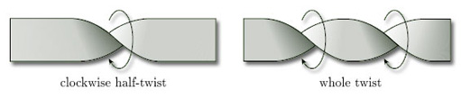
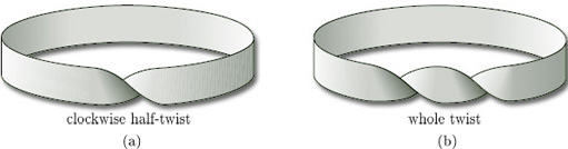
We say that the band shown on the left of Figure 47 has a half-twist – and going from left to right it is a clockwise half-twist – while the band on the right has two clockwise half-twists, making a whole twist. A half-twist is through ![]() radians; a whole twist is through 2
radians; a whole twist is through 2![]() radians.
radians.
Clearly, the twists must be in the same direction (clockwise or anticlockwise), or they will cancel each other out, as Figure 48 shows.
If we join up the ends of a band with a half-twist, we get a Möbius band, as shown in Figure 49(a). But what do we get if we join up the ends of a band with a whole twist, as in Figure 49(b)?
To answer this question, we cut the band, as shown in Figure 50. We can then undo the whole twist, glue the cut edges back together (making sure that the two edges are in the same direction, as before), and obtain a cylinder.
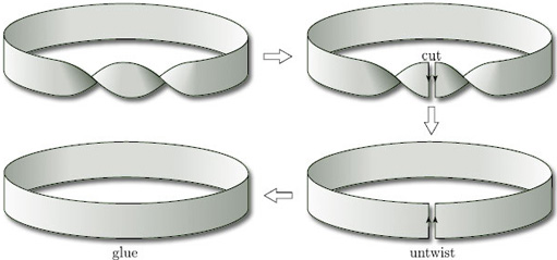
This cutting and gluing process is an example of a homeomorphism, as we saw in Section 2.4. Thus:
a band with a whole twist is homeomorphic to a band with no twists.
Clearly, using the method outlined above, we can undo any number of whole twists, so that a band with any number of whole twists is homeomorphic to a band with no twists: a cylinder. However, we cannot undo a half-twist. Thus, for example, if we have a band with three whole twists and an extra half-twist, then we can untwist the three whole twists but we cannot do anything with the half-twist, so we have a Möbius band.
We can conclude that, topologically, there are just two types of band:
-
bands with an even number of half-twists, which are homeomorphic to a cylinder;
-
bands with an odd number of half-twists, which are homeomorphic to a Möbius band.
The intuitive difference we feel between a band with a number of twists and a band with no twists (cylinder) or one twist (Möbius band) is captured by a theorem which states that the homeomorphisms between such bands cannot be extended to homeomorphisms of ![]() 3.
3.
This categorisation of bands will prove useful when we discuss orientability in Section 3.2.
Problem 11
Write down the boundary number β of a band with:
(a) three half-twists; (b) four half-twists.
Answer
(a) β = 1; (b) β = 2.
3.1.1 Inserting half-twists
We can insert half-twists into a paper surface whenever a piece of the surface is homeomorphic to a rectangle ABCD with the following properties:
the edges AB and CD of the rectangle map to distinct parts of the boundary of the surface, and the edges BC and DA of the rectangle map to non-boundary points of the surface.
As illustrated in Figure 51, the process of inserting a half-twist consists of cutting out the rectangle, giving it a half-twist so that the edge DA appears as it was but the edge BC is in the opposite direction, and then gluing it back.
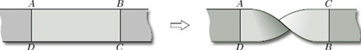
Since inserting a half-twist is not a homeomorphism, this process allows us to create new surfaces.
As well as creating a new surface, inserting a half-twist can change the boundary number. For example, Figure 52(a) shows a paper surface with boundary number β = 3. If we give the marked rectangle a half-twist, as shown on the right, then we obtain a surface with boundary number β = 2.
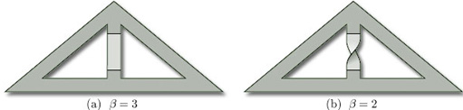
Problem 12
Starting with the paper surface shown in Figure 52(b), insert a half-twist to produce a surface with boundary number β = 1.
Answer
One way to insert a half-twist to obtain a surface with boundary number β = 1 is the following:
3.2 Orientability
The idea of orientability is another fundamental concept that we need for the study of surfaces. To illustrate the underlying idea, we consider two familiar surfaces – a cylinder and a Möbius band.
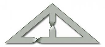
We can distinguish between a cylinder and a Möbius band by noticing that every cylinder has an ‘inside’ and an ‘outside’, as shown in Figure 53, and we can paint one red and the other blue. But if we try to paint a Möbius band in two colours, we fail – it has just one ‘side’. Equivalently, an ant crawling on a Möbius band can visit all points of the surface without crossing the boundary edge, whereas an ant on a cylinder can visit only the inside or the outside without crossing the boundary edges.
Two-sided surfaces in space, such as a cylinder, are examples of orientable surfaces, whereas one-sided surfaces in space, such as a Möbius band, are examples of non-orientable surfaces.
An orientable surface is one where consistent ‘orientation’ can be assigned over the entire surface; a non-orientable surface is one where this cannot be done.
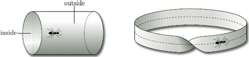
To see what we mean by this, let us take a cylinder and place on its surface a clock face whose minute hand is fixed at 12 and whose hour hand is fixed at 3, as shown in Figure 54(a): notice that the hour hand is found by going through ![]() /2 radians clockwise from the minute hand.
/2 radians clockwise from the minute hand.
If we now slide the clock face along any closed curve on the surface, keeping the hour hand pointing along the curve, then the hour hand is always ![]() /2 radians clockwise from the minute hand: for example, if the hour hand moves along the curve C shown in Figure 54(b), then the clock face continues to show 3 o'clock. This means that we can consistently define ‘clockwise’ at any point of the surface: the hour hand is always
/2 radians clockwise from the minute hand: for example, if the hour hand moves along the curve C shown in Figure 54(b), then the clock face continues to show 3 o'clock. This means that we can consistently define ‘clockwise’ at any point of the surface: the hour hand is always ![]() /2 radians clockwise from the minute hand.
/2 radians clockwise from the minute hand.
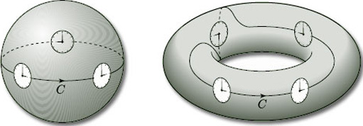
A similar situation occurs if we slide a clock face along any closed curve C on the surface of a sphere or a torus, as shown in Figure 55: in each case the hour hand is always ![]() /2 radians clockwise from the minute hand, and so we can again define ‘clockwise’ consistently.
/2 radians clockwise from the minute hand, and so we can again define ‘clockwise’ consistently.
Orientable surfaces are surfaces for which we can define ‘clockwise’ consistently: thus, the cylinder, sphere and torus are orientable surfaces. In fact, any two-sided surface in space is orientable: thus the disc, cylinder, sphere and n-fold torus, all with or without holes, are orientable surfaces.
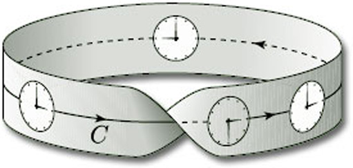
Let us now consider a clock face on a Möbius band, and let us slide it around the central curve C, as shown in Figure 56. Starting from any point on the curve, the twist in the surface causes the clock face to be upside-down when it first returns to that point: the hour hand still points to 3, but the minute hand now points downwards. Thus, the hour hand is no longer ![]() /2 radians clockwise from the minute hand. This means that we cannot consistently define ‘clockwise’ at every point of a Möbius band. Thus, the Möbius band is a non-orientable surface. In fact, any one-sided surface in space is non-orientable.
/2 radians clockwise from the minute hand. This means that we cannot consistently define ‘clockwise’ at every point of a Möbius band. Thus, the Möbius band is a non-orientable surface. In fact, any one-sided surface in space is non-orientable.
As we shall soon see, the Klein bottle and projective plane are also non-orientable.
Just as we use the boundary number β to distinguish between surfaces without boundary (β = 0) and surfaces with boundary (β > 0), so we introduce a number that distinguishes between orientable and non-orientable surfaces. This is another of the three characteristic numbers we use to classify compact surfaces.
Definition
The orientability number ω of a surface is:
-
0 if the surface is orientable;
-
1 if the surface is non-orientable.
(ω is the Greek letter omega.)
For example, ω = 0 for the disc, cylinder, sphere and n-fold torus, all with or without holes, and ω = 1 for the Möbius band.
As you might expect, we have the following result, which tells us that the orientability number is a topological invariant.
Theorem 3
Two surfaces that are homeomorphic have the same orientability number.
(We omit the proof, which is beyond the scope of this course.)
Problem 13
Write down the orientability number ω of each of the following surfaces:
(a) the 3-fold torus; (b) a band with three half-twists.
Answer
(a) ω = 0
(b) A band with three half-twists is homeomorphic to a Möbius band, and so, by Theorem 3, ω = 1.
One way of determining the orientability number of a given surface is to ascertain whether the surface contains a Möbius band.
Theorem 4
A surface that contains no Möbius band is orientable (ω = 0).
A surface that contains a Möbius band is non-orientable (ω = 1).
(We omit the proof, which is beyond the scope of this course.)
3.2.1 Remarks
-
By ‘contains’, we mean that we can find part of the surface that is homeomorphic to a Möbius band. The edge of the Möbius band does not need to correspond to an edge at the surface, so that a surface without boundary can be non-orientable (as we shall shortly see).
-
When seeking Möbius bands in a surface, it can be helpful to look at all possible closed curves on the surface and thicken these into bands.
-
Remember, from Section 3.1, that all bands with an odd number of half-twists (in the same direction) are homeomorphic to Möbius bands.
Worked problem 2
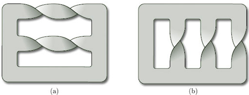
Determine whether each of the paper surfaces in Figure 57 is orientable.
Solution
(a) The top and middle of this surface have two half-twists each. These can be cut and glued back together to give the surface in Figure 58.
This surface is a disc with 2 holes, which is orientable (ω = 0).
(b) This surface contains several Möbius bands, two of which correspond to the closed curves shown in Figure 59.
The surface is therefore non-orientable (ω = 1).
Problem 14
Answer
(a) This surface contains a Möbius band, indicated by the closed curve, so is non-orientable (ω = 1).
(b) This surface contains no Möbius bands, so is orientable (ω = 0).
(c) This surface contains several Möbius bands, one of which is indicated by the closed curve, so is non-orientable (ω = 1).
Theorem 4 can be applied to all types of surface, not just paper surfaces. It can even be applied to representations of surfaces as polygons with edge identifications, as we shall see in Section 3.3, where we show that the projective plane and the Klein bottle are non-orientable.
3.3 The projective plane
We now consider one of the most important non-orientable surfaces – the projective plane (sometimes called the real projective plane). In Section 2 we introduced it as the surface obtained from a rectangle by identifying each pair of opposite edges in opposite directions, as shown in Figure 61. The projective plane is of particular importance in relation to the classification of surfaces – the Classification Theorem can be interpreted as saying that all surfaces without boundary can made from a sphere by adjoining either toruses or projective planes.
You may already be familiar with a geometric way of viewing the projective plane. This gives a completely different way of thinking about it: indeed, it is not even immediately obvious from the geometric approach why it is a surface!
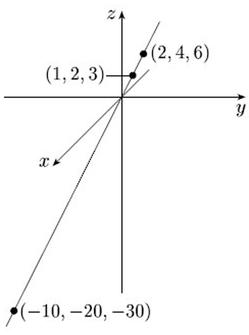
The geometric approach is to define the projective plane as the set of all infinite lines through the origin in Euclidean three-dimensional space: this means that each infinite line through the origin is to be regarded as a ‘point’ of the projective plane. To do this, we take ![]() 3, remove the origin (0, 0, 0), and consider any two of the remaining points (x, y, z) and (x', y', z') of
3, remove the origin (0, 0, 0), and consider any two of the remaining points (x, y, z) and (x', y', z') of ![]() 3 to be equivalent if and only if they lie on the same infinite line through the origin – that is, x' = kx, y' = ky, z' = kz, for some non-zero real number k. For example, the points (1, 2, 3), (2, 4, 6) and (−10, −20, −30) of
3 to be equivalent if and only if they lie on the same infinite line through the origin – that is, x' = kx, y' = ky, z' = kz, for some non-zero real number k. For example, the points (1, 2, 3), (2, 4, 6) and (−10, −20, −30) of ![]() 3 are all equivalent points, as Figure 62 illustrates. Each set of equivalent points, together with the point (0, 0, 0), comprises an infinite line through the origin and is thus a ‘point’ of the projective plane, which we refer to as a projective point. We denote a projective point using square brackets around the coordinates of a representative point on the infinite line: thus the projective point containing the points (1, 2, 3), (2, 4, 6) and (−10, −20, −30) may be written as [1, 2, 3] or [2, 4, 6] or indeed as [k, 2k, 3k] for any non-zero number k.
3 are all equivalent points, as Figure 62 illustrates. Each set of equivalent points, together with the point (0, 0, 0), comprises an infinite line through the origin and is thus a ‘point’ of the projective plane, which we refer to as a projective point. We denote a projective point using square brackets around the coordinates of a representative point on the infinite line: thus the projective point containing the points (1, 2, 3), (2, 4, 6) and (−10, −20, −30) may be written as [1, 2, 3] or [2, 4, 6] or indeed as [k, 2k, 3k] for any non-zero number k.
Problem 15
Which of the following points (x, y, z) of ![]() 3 correspond to the same projective points [x, y, z]?
3 correspond to the same projective points [x, y, z]?
(3, −1, 2), (4, −2, 6), (−9, 3, −6), (12, −6, −9), (15, −5, 10), (−18, 9, −27).
Answer
(3, −1, 2), (−9, 3, −6) and (15, −5, 10) correspond to the projective point [3, −1, 2]. (4, −2, 6) and (−18, 9, −27) correspond to the projective point [4, −2, 6] = [2, −1, 3]. (12, −6, −9) corresponds to the projective point [12, −6, −9] = [4, −2, −3].
This definition of the projective plane is no more helpful than the definition in terms of a rectangle with edge identifications as a means of picturing what the projective plane really looks like. It does, however, lead us towards a description of the projective plane in which each projective point looks like a point of ![]() 3. We begin by enclosing the origin within the sphere of unit radius, as shown in Figure 63. Each infinite line through the origin gives rise to a diameter of this sphere which meets the sphere in exactly two antipodal points, (p, q, r) and (−p, −q, −r). So we can think of the projective plane as the set of all these pairs of antipodal points on the unit sphere, and the projective point [p, q, r] now corresponds to the two points (p, q, r) and (−p, −q, −r) of
3. We begin by enclosing the origin within the sphere of unit radius, as shown in Figure 63. Each infinite line through the origin gives rise to a diameter of this sphere which meets the sphere in exactly two antipodal points, (p, q, r) and (−p, −q, −r). So we can think of the projective plane as the set of all these pairs of antipodal points on the unit sphere, and the projective point [p, q, r] now corresponds to the two points (p, q, r) and (−p, −q, −r) of ![]() 3 on the sphere. This gives a natural ‘two-to-one’ map from the sphere to the projective plane which sends the two points (p, q, r) and (−p, −q, −r) to the projective point [p, q, r].
3 on the sphere. This gives a natural ‘two-to-one’ map from the sphere to the projective plane which sends the two points (p, q, r) and (−p, −q, −r) to the projective point [p, q, r].
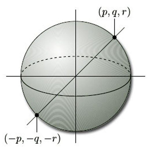
This sphere has equation![]()
So we can regard the projective plane as made up of pairs of points on the sphere. If we could systematically select a single point from each of these pairs, then we would have an even better picture of the projective plane. Unfortunately, there is no natural way of thinking of exactly half of the points on a sphere. We can certainly think of the points [p, q, r] with r ≠ 0 as lying on the upper hemisphere: we simply associate with each projective point [p, q, r] whichever of the two points (p, q, r) and (−p, −q, −r) on the sphere has its third coordinate positive. But if r = 0 then we have a problem: the projective point [p, q, r] is associated with both the points (p, q, 0) and (−p, −q, −0) of the sphere, and there is no satisfactory way of choosing just one of them.
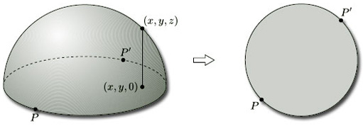
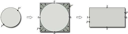
Instead, we proceed as follows. We first represent the projective plane as the upper hemisphere with antipodal pairs of points on the equator (r = 0) identified. We then map this space on to the unit disc by projecting vertically downwards, using the map (x, y, z) ![]() (x, y, 0), as shown in Figure 64. We thereby represent the projective plane as a disc with antipodal points P and P' on the boundary identified.
(x, y, 0), as shown in Figure 64. We thereby represent the projective plane as a disc with antipodal points P and P' on the boundary identified.
Finally, we project this disc radially onto a circumscribing square. This represents the projective plane as a square with diagonally opposite points P and P' on the boundary identified, as shown in Figure 65. By stretching the square to a rectangle, we obtain our earlier description of the projective plane as a rectangle with opposite edges identified in opposite directions.
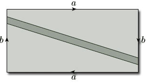
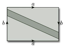
In Section 3.2 we asserted that a surface is non-orientable if it contains a Möbius band. To show that the projective plane is non-orientable, we consider its representation as a rectangle with opposite edges identified in opposite directions, as shown in Figure 66. When we identify the edges labelled b, the shaded strip becomes a Möbius band. This shows that the projective plane contains a Möbius band, and therefore by Theorem 4 is non-orientable.
Problem 16
Use the Klein bottle's representation as a rectangle with edge identifications (see Figure 31) to show that it is non-orientable.
Answer
The Klein bottle's representation as a rectangle with edge identifications is shown below. When we identify the edges labelled b, the shaded strip becomes a Möbius band, and thus by Theorem 4 the Klein bottle is non-orientable.
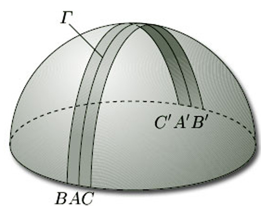
We can obtain the same result using the representation of the projective plane as an upper hemisphere with antipodal points identified. To do so, we draw half of a great circle Γ on it through two antipodal points A, A' and the north pole. We then ‘fatten’ this line to a narrow strip that meets the equator at the pairs of antipodal points B, B' and C, C', as shown in Figure 67. The boundary of this strip around Γ is a single curve, and the shaded strip is a Möbius band, showing that the surface is non-orientable. Either way, the presence of a Möbius band shows that the projective plane is non-orientable. This result is so important that we state it as a theorem.
Theorem 5
The projective plane is non-orientable.
If we remove a Möbius band from the projective plane, what remains? Using the rectangle representation, we first obtain two pieces, as shown in Figure 68(a), with the edges labelled a, b and c to be identified in pairs; the edges x and y form the boundary of the removed Möbius band. Turning each piece over and identifying the edges labelled a, we obtain Figure 68(b). Identifying the edges labelled b and then the edges labelled c, we obtain a purse-like object whose boundary is the boundary of the Möbius band, as shown in Figure 68(c). Finally, if we open the purse and flatten it out, we obtain a disc whose boundary is the boundary of the Möbius band, as shown in Figure 68(d).
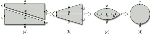
Thus, removing a Möbius band from the projective plane yields a disc whose boundary is the boundary of the Möbius band. Gluing the Möbius band back again leads to the following surprising conclusion.
Theorem 6
The projective plane is obtained by gluing a disc and a Möbius band along their boundaries.
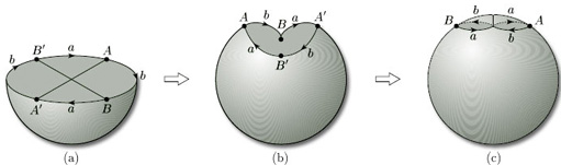
We can use this result to provide us with an alternative picture of a Möbius band. We begin with a representation of the projective plane as a hemisphere. However, instead of taking the upper hemisphere as before, it is now more convenient to represent it as the lower hemisphere, but again with antipodal points on the equation identified, as shown in Figure 69(a). We then distort the hemisphere slightly, giving the equator a ‘flower’ shape, as shown in Figure 69(b): this makes it easier for us to see what is to be identified with what. We see that the edge AB is to be identified with the edge A'B', and that the edge BA' is to be identified with the edge B'A. We can perform either one of these two identifications without too much difficulty after some judicious stretching of the surface; but, when we try to perform the other, we need to let the surface ‘intersect itself along a line, the vertical line in Figure 69(c).
Thus Figure 69(c) gives us a representation of the projective plane in which no identifications need to be made, but it is not a representation in ![]() 3 since the surface pictured intersects itself.
3 since the surface pictured intersects itself.
We saw a similar picture of the Klein bottle, as a surface that intersects itself, in Figure 31.
If we now remove a disc from the surface in Figure 69(c), as shown in Figure 70, Theorem 4 tells us that what we have left is a Möbius band. This new picture of a Möbius band is called a cross-cap, from its supposed resemblance to a bishop's mitre.
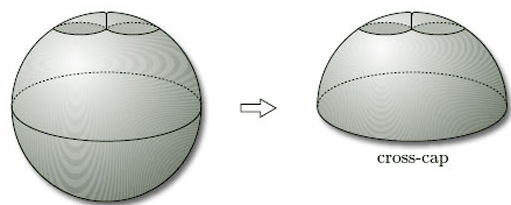
In general, we add a cross-cap to a surface by removing a disc and identifying opposite points on the boundary (or by identifying the boundary curve with that of a Möbius band). Adding one cross-cap to the sphere gives the projective plane; adding two cross-caps to the sphere gives the Klein bottle.
We stated in Section 2 that neither the projective plane nor the Klein bottle are surfaces in space. In both cases, whenever all identifications are made, the resulting representation is a surface that intersects itself and so cannot be embedded in ![]() 3. In fact, a non-orientable surface can be represented as a surface in space if and only if it has a boundary.
3. In fact, a non-orientable surface can be represented as a surface in space if and only if it has a boundary.
Theorem 7
A non-orientable surface can be represented as a surface in space if and only if it has a boundary.
(We omit the proof, which is beyond the scope of this course.)
We also have the following result:
Theorem 8
All orientable surfaces can be represented as surfaces in space.
(We omit the proof, which is beyond the scope of this course.)
So the extra freedom that we gain by studying surfaces in general, and not just surfaces in space, is precisely the freedom to study non-orientable surfaces without boundary, of which the projective plane and the Klein bottle are the most important examples.
4 The Euler characteristic
4.1 Nets on surfaces
In Section 4 we introduce the third of the numbers we associate with a surface – the Euler characteristic. This is used in the Classification Theorem, which we state at the end of the section. To define the Euler characteristic, we need the idea of a subdivision of a surface, which we introduce by first considering the informal idea of a net on a surface.
To define the Euler characteristic, we need the idea of covering a surface with a net of polygons. To explain what we mean let us look at some examples.
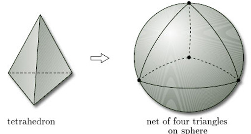
We start with a sphere and draw triangles upon it. One way to do this is to start with a tetrahedron, which (when considered as a polyhedral surface) is homeomorphic to the sphere. If we now ‘inflate’ the tetrahedron to obtain a sphere, the four triangular faces of the tetrahedron create a net of four triangles on the sphere, as Figure 71 illustrates. Here the word ‘triangle’ means any three-sided region drawn on a surface. They usually have curved sides and are not flat.
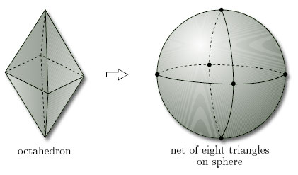
We can similarly inflate an octahedron, as shown in Figure 72.
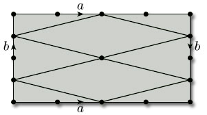
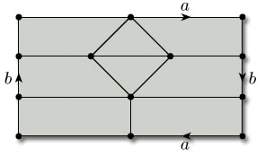
We can also draw nets of triangles on other surfaces, such as the torus, for which it is convenient to show the net on the representation of the torus as a rectangle with edge identifications, as in Figure 73.
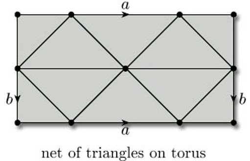
Remember that here the edge identifications a and b apply to the whole of the horizontal and vertical edges of the rectangle. For the sake of clarity, we assume that all parts of the edges of the defining polygon correspond to edges of the net.
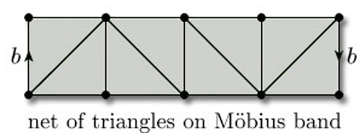
When we draw triangles on a surface with boundary, unless stated otherwise, we require that the boundary is decomposed into edges that are edges of the triangles. For example, Figure 74 shows a net of triangles on a Möbius band, again shown as a rectangle with edge identifications.
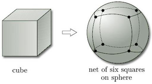
We need not restrict our attention to triangles: we can use polygons with any number of sides. For example, a cube can be inflated to give us a net of squares on a sphere, as Figure 75 shows.
We can also use different types of polygon on the same surface. Figure 76 shows a net of triangles and quadrilaterals on a sphere, obtained by inflating a polyhedron called the cuboctahedron.
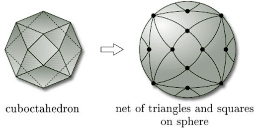
The surfaces we are considering include both surfaces in space and surfaces that cannot be represented in ![]() 3, such as the Klein bottle and the projective plane. For example, Figure 77 shows a net of quadrilaterals on a Klein bottle, shown as a rectangle with edge identifications. Note that the faces that look like triangles are actually quadrilaterals, since each has four vertices and four edges.
3, such as the Klein bottle and the projective plane. For example, Figure 77 shows a net of quadrilaterals on a Klein bottle, shown as a rectangle with edge identifications. Note that the faces that look like triangles are actually quadrilaterals, since each has four vertices and four edges.
Problem 17
Draw an example of each of the following nets:
-
(a) a net of quadrilaterals on a torus;
(b) a net of triangles on a projective plane.
Answer
Examples of suitable nets are the following. In each case we draw the net on the surface represented as a rectangle with edge identifications.
4.2 Subdivisions
In this subsection we formalise the idea of a net by introducing a useful concept called a subdivision of a surface. This is a standard kind of net drawn on a surface, and is defined in terms of vertices, edges and faces. It leads to the idea of the Euler characteristic of the surface.
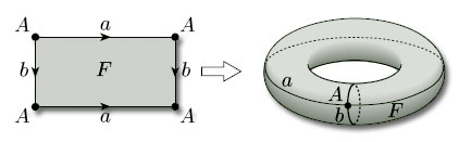
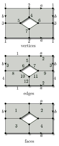
All surfaces obtained from polygons by identifying edges arise from a net (of sorts) consisting of a single polygonal face, together with the edges and vertices that remain after the identifications have been carried out. For example, a torus is obtained from a rectangle by identifying edges: the top and bottom edges become the same, the left and right edges become the same, the four vertices of the rectangle become the same, and there is just one face, as shown in Figure 78. This ‘net’ therefore has one vertex (A), two edges (a and b) and one face (F): the face F is what is left after all the vertices and edges have been removed.
We now try to formalise the idea of a net of polygons on a surface so as to include both this case and the nets described in the previous subsection: the result is called a subdivision of the surface. We start with the surface and mark a set of vertices (points) on it, joining them by edges (non-crossing curves) to produce a connected graph, as shown in Figure 79(a). If we now remove the vertices and edges of this graph from the surface, as shown in Figure 79(b), then their complement splits into a finite number of pieces. If these pieces are all homeomorphic to open discs, then the vertices and edges define a subdivision of the surface, and the disc-like regions are the faces of the subdivision.
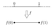
Before we can write down a formal definition of a subdivision of a surface, we must formalise the idea of an edge: an edge of a subdivision is the image of the open interval (0, 1) under a one-one continuous map f of the closed interval [0, 1], as Figure 80 illustrates. The points f(0) and f(1) are the endpoints of the edge. (The endpoints are not part of the edge and may coincide.)
Definition
A subdivision of a surface consists of a finite set of points, called vertices, and a finite set of edges, as defined above, such that:
-
each vertex is an endpoint of at least one edge;
-
each endpoint of an edge is a vertex;
-
the vertices and edges form a connected graph;
-
no two edges have any points in common;
-
if the surface has a boundary, the boundary consists only of vertices and edges;
-
the space obtained from the surface by removing the vertices and edges is a union of disjoint pieces, called faces, each of which is homeomorphic to an open disc.
An example of a subdivision is the ‘cube subdivision’ of a sphere, shown in Figure 81, which has 8 vertices, 12 edges and 6 faces.
It is natural to say that two adjacent faces ‘meet along their common edge’, and that edges ‘meet at a vertex’, but strictly speaking this is incorrect since the vertices, edges and faces of a subdivision are disjoint.
To allow us to use such natural phrases, we shall say that:
-
a vertex belongs to an edge if every open set containing the vertex contains points of the edge, so the vertex is in the closure of the edge;
-
a vertex belongs to a face if every open set containing the vertex contains points of the face, thus the vertex is in the closure of the face;
-
an edge belongs to a face if every open set containing the edge contains points of the face, thus the edge is in the closure of the face.
These relationships are illustrated in Figure 82. They allow us to say that two edges or faces meet at a vertex if there is a vertex that belongs to both of them, and that two faces meet at an edge if there is an edge that belongs to both of them. They also allow us to say that a face has a number of edges and vertices, namely those edges and vertices that belong to it. We shall also say that the edges that meet at a vertex are the incident edges of that vertex.
To illustrate this terminology, consider the subdivision of a closed disc shown in Figure 83, which has 5 vertices (A, B, C, D, E), 7 edges (AB, AC, AD, AE, BC, BD, BE) and 3 faces (1, 2, 3). Faces 1 and 2 meet at edges AD and BD and at vertices A, B and D; faces 2 and 3 meet at edge AB and at vertices A and B; faces 1 and 3 meet only at vertices A and B. Edges AC and BC meet at vertex C; edges AC and AD meet at vertex A; edges AD and BC do not meet; and so on. Face 1 has 4 edges (AC, AD, BC, BD) and 4 vertices (A, B, C, D); face 2 has 3 edges (AB, AD, BD) and 3 vertices (A, B, D); face 3 has 3 edges (AB, AE, BE) and 3 vertices (A, B, E).
Problem 18
List the vertices, edges and faces of each of the subdivisions of a closed disc in Figure 84. Describe where face 1 meets the other faces in each case. How many edges and vertices does face 3 have in each case?
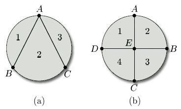
Answer
(a) vertices {A, B, C},
edges {AB (twice), AC (twice), BC};
faces {1, 2 ,3}.
Faces 1 and 2 meet at the inner edge AB and at vertices A and B. Faces 1 and 3 meet at vertex A only. Face 3 has 2 edges (both from A to C) and 2 vertices (A and C).
(b) vertices {A, B, C, D, E},
edges {AB, BC, CD, DA, AE, BE, CE, DE},
faces {1, 2, 3, 4}.
Faces 1 and 2 meet at the edge AE and at vertices A and E. Faces 1 and 3 meet at vertex E only. Faces 1 and 4 meet at edge DE and at vertices D and E. Face 3 has 3 edges (BC, BE, CE) and 3 vertices (B, C and E).
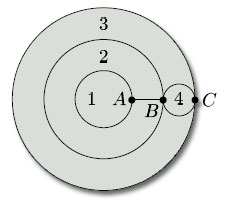
We noted earlier that the endpoints of an edge may coincide. This means that an edge can meet itself, as is illustrated by the circular edges in the subdivision of a closed disc shown in Figure 85. This figure also shows that a face may meet itself along an edge – face 2 meets itself along the edge AB (and of course at the vertices A and B) – and also a face may meet itself at a vertex or vertices but not along an edge – face 3 meets itself at vertices B and C only.
From the definition of a subdivision and the examples we have given, we may deduce the following properties of subdivisions of surfaces:
-
each point of the surface must be a vertex, or lie on an edge, or lie in a face;
-
faces meet only at vertices and edges;
-
two faces may meet at one or more vertices;
-
two faces may meet at one or more edges;
-
edges meet only at vertices;
-
an edge may belong to one or two faces;
-
an edge may have one or two vertices;
-
a vertex may belong to one or more faces;
-
a vertex may belong to one or more edges.
4.3 The Euler characteristic
Subdivisions of surfaces lead to the third number used to classify surfaces, the Euler characteristic.
Definition
The Euler characteristic χ of a subdivision of a surface is

where V, E and F denote (respectively) the numbers of vertices, edges and faces in the subdivision.
Remark
The formula χ = V − E + F is often referred to as Euler's Formula.
For example, the tetrahedron gives rise to a subdivision of the sphere where the vertices, edges and faces of the tetrahedron correspond to the vertices, edges and faces of the subdivision (Figure 86). This subdivision has 4 vertices, 6 edges and 4 faces, so its Euler characteristic is
Similarly, the cube gives rise to a subdivision of the sphere (Figure 87).
This subdivision has 8 vertices, 12 edges and 6 faces, so its Euler characteristic is
Figure 88 shows a subdivision of a closed disc, with 3 faces, 5 vertices and 7 edges. Its Euler characteristic is

We saw in the last subsection that the rectangle with edge identifications that define a torus (Figure 89) represents a subdivision of the torus, with 1 vertex, 2 edges and 1 face. Its Euler characteristic is
As the last example indicates, when we are dealing with a surface defined by a polygon with edge identifications, we need to be careful how we count the vertices, edges and faces. The following worked problem provides further illustration.
Worked problem 3
Problem 19
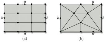
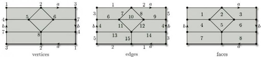
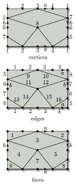
Find the Euler characteristic of each of the subdivisions in Figure 92: (a) torus with 1 hole, (b) Möbius band, (c) Klein bottle.
Answer
(a) This subdivision has 7 vertices, 12 edges, and 4 faces, so its Euler characteristic is
(b) This subdivision has 8 vertices, 16 edges, and 8 faces, so its Euler characteristic is

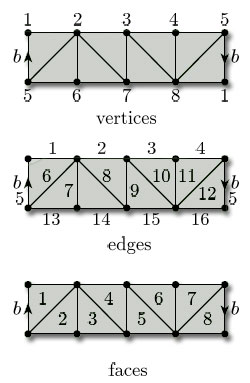
(c) This subdivision has 8 vertices, 16 edges, and 8 faces, so its Euler characteristic is
We have seen that the Euler characteristics of tetrahedral and cubic subdivisions of the sphere are equal to 2. More generally, it can be shown that the Euler characteristic is the same for any two subdivisions of the same surface. The proof of this general result is difficult, and so we simply state the result here.
Theorem 9
Any two subdivisions of the same surface have the same Euler characteristic.
For example, every subdivision of the sphere has Euler characteristic 2. Similarly, we have seen a subdivision of the torus with Euler characteristic 0: it follows that every subdivision of the torus has Euler characteristic 0.
Theorem 9 allows us to speak of the Euler characteristic of a surface, independently of the choice of subdivision, and to compute it using the most convenient subdivision.
Our assumption that the surface is compact guarantees that the Euler characteristic is always finite.
Definition
The Euler characteristic of a surface S is the Euler characteristic of any subdivision of S. It is denoted by χ(S).
(χ is the Greek letter chi.)
The earlier examples now enable us to conclude that the Euler characteristic of the sphere is 2, of the closed disc is 1, of the torus is 0, of the projective plane is 1, of the torus with 1 hole is −1, of the Möbius band is 0 and of the Klein bottle is 0.
Problem 20
By considering the subdivisions in Figure 93, verify the Euler characteristic of each of the given surfaces.
Answer
(a) This subdivision has 7 vertices, 12 edges, and 6 faces, so the Euler characteristic is
(b) This subdivision has 5 vertices, 10 edges, and 5 faces, so the Euler characteristic is
(c) This subdivision has 6 vertices, 15 edges, and 10 faces, so the Euler characteristic is

Problem 21
By drawing a suitable subdivision, find the Euler characteristic of a cylinder.
Answer
A simple subdivision is shown below. It has 2 vertices, 3 edges and 1 face, so the Euler characteristic is

We conclude this subsection by remarking that any homeomorphism of a surface S onto a surface S' maps a subdivision of S onto a subdivision of S', sending the vertices of S to vertices of S', the edges of S to edges of S', and the faces of S to faces of S', in a one-to-one fashion. It follows that the value of V − E + F remains unchanged, and therefore that the Euler characteristic of a subdivision is preserved under homeomorphisms. Thus the Euler characteristic of a surface is a topological invariant.
4.4 Historical note on the Euler characteristic
A little history is instructive here, because it shows how difficult Theorem 9 really is. By 1900 the classification of compact surfaces was well understood, although proofs of the major theorems relied more on intuition than would be acceptable today. Attention switched to objects called ‘3-manifolds’, topological spaces each point of which has a neighbourhood homeomorphic to the interior of the unit ball in ![]() 3. The French mathematician Henri Poincaré – one of the leading mathematicians of his time – was among the first to study spaces of three or more dimensions. He proposed to study 3-manifolds by triangulating them – that is, by subdividing them into tetrahedra. Faced with the three-dimensional version of the problem of finding properties of a 3-manifold that are independent of any triangulation, he conjectured that given any two triangulations, there is a further triangulation which contains both. But not even he could prove it. His conjecture stood until 1948, and the corresponding result for
3. The French mathematician Henri Poincaré – one of the leading mathematicians of his time – was among the first to study spaces of three or more dimensions. He proposed to study 3-manifolds by triangulating them – that is, by subdividing them into tetrahedra. Faced with the three-dimensional version of the problem of finding properties of a 3-manifold that are independent of any triangulation, he conjectured that given any two triangulations, there is a further triangulation which contains both. But not even he could prove it. His conjecture stood until 1948, and the corresponding result for ![]() 2 was proved only in 1963.
2 was proved only in 1963.
Perhaps the most eloquent indication of the difficulty of the proof of Theorem 9 was the remarkable discovery (by the American mathematician John Milnor in 1961) that the corresponding conjecture is false for spaces of dimension 6: this means that any proof in three dimensions must use some special property of three-dimensional space. This was one of a number of achievements for which Milnor received the Fields Medal in 1962, often regarded as the mathematical equivalent of the Nobel Prize.
Because of these difficulties, and even before Milnor's refutation of the general conjecture, a way had been found of avoiding it and working systematically in any number of dimensions. The method was pioneered in 1926 by another major mathematician, the Russian P.S. Alexandrov. His 600-page treatise Combinatorial Topology treats surfaces in Chapter III. You may find it consoling that he does not prove the invariance of the Euler characteristic in that chapter, but writes:
In contrast with the rest of the book, a great deal of the material in Chapter III depends on certain invariance theorems, which are not proved until Chapters V and X and are merely stated in this chapter … This procedure seems to me legitimate, since the proofs of these invariance theorems given subsequently are independent of the results of Chapter III. Otherwise, the exposition of the topology of surfaces would have to be postponed until much later, or burdened with a proof of invariance for the special case of two dimensions.
In short, one of the creators of the modern theory thought it best to teach surfaces with less than complete rigour, rather than burden his readers with proofs that were different in spirit from the pure study of surfaces. (He gave a rigorous proof many pages later.) Indeed, no undergraduate textbook author presents a rigorous treatment that does not take the reader on a long journey, finding that an intuitive grasp of the topic is all that is needed at this level and that it is entirely reliable.
4.5 Some general results
We next establish some general results about Euler characteristics. We start with a theorem that tells us what happens to the Euler characteristic of a surface when we remove an open disc.
Theorem 10: Disc Removal Theorem
The Euler characteristic of a surface with an open disc removed is one less than the Euler characteristic of the original surface.
Outline proof: Suppose that we are given a surface S containing an open disc. Any subdivision of S with the disc removed gives rise to a subdivision of S with the disc reinstated, as shown in Figure 94, and these two subdivisions have the same number V of vertices and the same number E of edges.
Recall that if a surface has a boundary then the boundary must consist of vertices and edges of the subdivision.
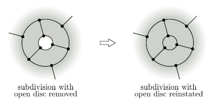
When we reinstate the disc, we increase F, the number of faces, by 1, while V and E are unchanged. So we increase the Euler characteristic χ = V − E +F by 1. It follows that the Euler characteristic of the surface with the disc removed is one less than the Euler characteristic of the original surface
The full proof is rather complicated, so we provide just an outline.
4.5.1 Surfaces with holes
Using this result, we can obtain the Euler characteristic of a surface with any number of holes by successively inserting the holes one at a time. For example, since a closed disc has Euler characteristic 1, it follows that a closed disc with 1 hole has Euler characteristic 0, a disc with 2 holes has Euler characteristic −1, and so on.
Problem 22
Use the above approach to determine the Euler characteristic of a torus with k holes.
Answer
Since a torus has Euler characteristic 0, it follows from Theorem 10 that a torus with 1 hole has Euler characteristic −1, a torus with 2 holes has Euler characteristic −2, and so on. In general, a torus with k holes has Euler characteristic −k.
Theorem 11
Inserting k holes into a surface reduces its Euler characteristic by k.
4.5.2 n-fold toruses
We can use a similar technique to find the Euler characteristic of a 2-fold torus. If we cut the surface into two, as shown in Figure 95, and separate the pieces, we obtain two copies of a 1-fold torus with 1 hole, each with Euler characteristic −1.
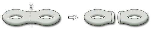
Consider any subdivision of the left-hand torus with 1 hole, and give the right-hand torus with 1 hole its mirror image subdivision. In this way, the vertices and edges on the boundary of each hole can be identified when we glue the two pieces back together. Note that the number of vertices on each boundary must be the same as the number of edges on that boundary.
Thus the vertices and edges on the boundaries contribute a value 0 to the Euler characteristic V − E + F of each piece, and also to the Euler characteristic of the 2-fold torus obtained by gluing the two pieces back together. Thus the Euler characteristic of the 2-fold torus is simply the sum of the Euler characteristics of the two pieces: (−1) + (−1) = −2.
We can carry out a similar procedure for a 3-fold torus. If we cut it into two pieces, as shown in Figure 96, we obtain a 2-fold torus with 1 hole and a 1-fold torus with 1 hole. The Euler characteristic of a 2-fold torus with 1 hole is (−2) − 1 = −3, by Theorem 10, and the Euler characteristic of a 1-fold torus with 1 hole is −1, so the Euler characteristic of a 3-fold torus is (−3) + (−1) = −4.
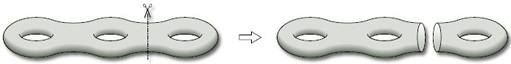
Continuing in this way, we obtain the Euler characteristic of an n-fold torus.
Theorem 12
The Euler characteristic of an n-fold torus is 2 − 2n.
We can also deduce the following theorem from the above discussion.
Theorem 13
The Euler characteristic of a surface obtained by gluing together two surfaces with boundary along a given boundary component of each is equal to the sum of the Euler characteristics of the original surfaces.
Problem 23
Find the Euler characteristic of the surface obtained by gluing a cylinder to a sphere with two holes, where each boundary of the cylinder is glued to the boundary of a separate hole.
Answer
A cylinder has Euler characteristic 0 and a sphere with two holes has Euler characteristic 2 − 2 = 0 (by Theorem 11). Therefore, by Theorem 13, the surface obtained by gluing these two surfaces together along the boundaries has Euler characteristic 0 + 0 = 0.
4.6 The Classification Theorem
In this subsection we state the Classification Theorem for surfaces, which classifies a surface in terms of its boundary number β, its orientability number ω and its Euler characteristic χ, each of which is a topological invariant – it is preserved under homeomorphisms.
Let us remind ourselves of these three numbers.
-
A surface may or may not have a boundary, and, if it does, then the boundary has finitely many disjoint pieces. The number of these boundary components is the boundary number β of the surface. (See Section 2.2.)
-
Some surfaces are orientable and some are not. The orientability number ω of a surface is 0 if the surface is orientable and 1 if it is non-orientable. (See Section 3.2.)
-
Surfaces can be subdivided, and for a given surface the Euler characteristic χ = V − E + F is independent of the subdivision used to compute it, and is therefore a property of the surface itself. (See Section 4.3.)
These three numbers β, ω and χ are collectively called the characteristic numbers of the surface.
Now, all three characteristic numbers are necessary for classifying surfaces since, for example:
-
a sphere and a torus both have β = 0 and ω = 0;
-
a torus and a Klein bottle both have β = 0 and χ = 0;
-
a torus and a cylinder both have ω = 0 and χ = 0.
It also turns out that these three numbers are sufficient to classify surfaces, and so we have the central result of this block.
Theorem 14: Classification Theorem for surfaces
Two surfaces are homeomorphic if and only if they have the same values for the characteristic numbers β, ω and χ.
4.6.1 Remarks
-
We already know that the characteristic numbers are topological invariants, that is, any two homeomorphic surfaces have the same values for the characteristic numbers. Thus it is solely the converse, namely if two surfaces have the same values for the characteristic numbers then they are homeomorphic, that we have to prove.
It follows from the Classification Theorem that if we restrict our attention to orientable surfaces (ω = 0), then the numbers β and χ characterise the surface completely – and similarly if we restrict our attention to non-orientable surfaces (ω = 1).
Our assumption that all surfaces are compact guarantees that the characteristic numbers are finite,
-
The Classification Theorem allows us to refer to the sphere, the torus, the Klein bottle, etc., rather than a sphere, a torus and a Klein bottle, etc.
Problem 24
Which surfaces are characterised by the following sets of characteristic numbers?
Answer
-
Sphere.
-
Möbius band.
-
Torus with 1 hole.
-
2-fold torus.
-
Projective plane.
Problem 25
Find the characteristic numbers of the surface obtained by gluing two Möbius bands along their boundaries. Deduce from the Classification Theorem that this surface is homeomorphic to the Klein bottle.
Answer
The surface obtained by gluing two Möbius bands together has no boundary components (β = 0), and is non-orientable (ω = 1). Also, by Theorem 13, its Euler characteristic is the sum of the Euler characteristics of each separate surface, so χ = 0 + 0 = 0. The Klein bottle has these values for its characteristic numbers, so (by the Classification Theorem) the glued surface is homeomorphic to the Klein bottle.
Worked problem 4
Find the characteristic numbers of the closed disc with two straps, shown in Figure 97.
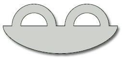
Solution
The surface has three boundary components, so β = 3. The surface contains no Möbius band, and is therefore orientable, so ω = 0. To find the Euler characteristic, we choose a subdivision. The one shown in Figure 98 has 8 vertices, 12 edges and 3 faces, so χ = 8 − 12 + 3 = −1.
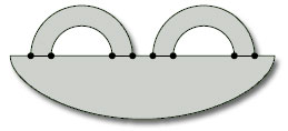
You could also argue that, as the surface is a closed disc with two holes, its Euler characteristic is 1 − 2= −1 (by Theorem 11).
Problem 26
Consider the closed disc with two straps added in other ways, sometimes with a twist, as shown in Figure 99. Compute the characteristic numbers of each surface, and then use the Classification Theorem to determine which of these surfaces are homeomorphic.
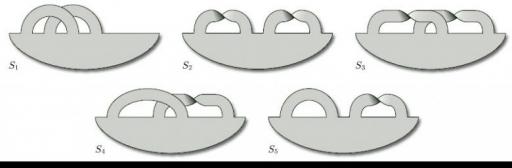
Answer
Each surface has a subdivision with 8 vertices, 12 edges and 3 faces, as indicated in Worked Problem 4. The Euler characteristic of each surface is therefore −1, as before.
The characteristic numbers β and ω are as follows.
| surface | S1 | S2 | S3 | S4 | S5 |
| β | 1 | 1 | 2 | 1 | 2 |
| ω | 0 | 1 | 1 | 1 | 1 |
It follows from the Classification Theorem that the surfaces S2 and S4 are homeomorphic, as are the surfaces S3 and S5; no other two surfaces are homeomorphic.
Problem 27
For each of the following paper surfaces, mark a subdivision and hence determine the characteristic numbers of the surface.
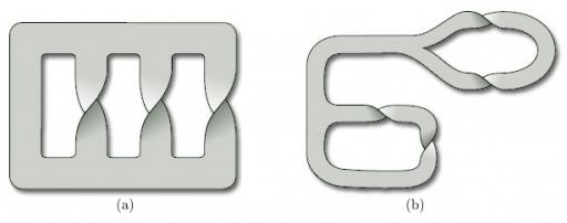
Answer
(a) We have drawn a subdivision with 12 vertices.
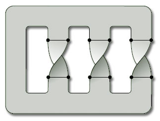
There are 18 edges and 4 faces, so the Euler characteristic is χ = 12 − 18 + 4 = −2.
There is one boundary component, so β = 1.
The surface is non-orientable (see Worked Problem 2(b)), so ω = 1.
(b) We have drawn a subdivision with 16 vertices.
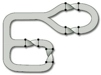
There are 24 edges and 7 faces, so the Euler characteristic is χ = 16 − 24 + 7= −1.
There are three boundary components, so β = 3.
The surface is orientable (see Solution 14(b)), so ω = 0.
For future reference, we conclude this section with a table of some common surfaces with their characteristic numbers.
| surface | β | ω | χ |
|---|---|---|---|
| sphere | 0 | 0 | 2 |
| n-fold torus | 0 | 0 | 2 − 2n |
| Klein bottle | 0 | 1 | 0 |
| projective plane | 0 | 1 | 1 |
| closed disc | 1 | 0 | 1 |
| cylinder | 2 | 0 | 0 |
| Möbius band | 1 | 1 | 0 |
In addition, adding a hole to any surface increases its boundary number β by 1, keeps its orientability number ω the same, and decreases its Euler characteristic χ by 1.
5 Edge identifications
5.1 Identifying edges of a polygon
In this section, we revisit the construction of surfaces by identifying edges of polygons, as described in Section 2. Recall that, if we take any polygon in the plane and identify some of its edges in pairs, then we obtain a surface. When specifying how a given pair of edges is to be identified, we choose one of the two possible relative orientations of these edges.
In diagrams we represent such a rule for identifying edges by labelling the edges with letters and arrowheads, as in Figure 101: a pair of edges is identified if each carries the same letter, and the direction of identification is indicated by the arrowheads. We refer to an edge labelled with an arrowhead as a directed edge. Any assignment of letters and arrowheads to edges in which a particular letter appears on exactly two directed edges defines a rule for identifying edges of a polygon.
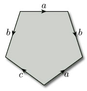
To prove that we do obtain a surface when we identify edges of a polygon in this way, we need to show how to make the resulting set into a topological space. We use a topology called the identification topology. We explore this topology and its consequences in this section.
5.2 The identification topology
Our aim is to show that the object that we produce when we identify some or all the edges of a polygon is a surface. Therefore, by the definition of a surface given in Section 2.5, we must show how it can be given the structure of a topological space, and that this space is Hausdorff. Furthermore, we must show that every point has a disc-like or half-disc-like neighbourhood. We shall address the issue of showing that the object is a topological space in this subsection. We shall consider neighbourhoods and show that the space is Hausdorff in Section 5.3.
[ Its compactness and path-connectedness are guaranteed by its method of construction. ]
Our method for showing that the object is a topological space will be to construct a bijection between it and a known topological space. This will then allow us to define open sets for the object and hence show that it is a topological space.
The obvious known topological space is the polygon with edge identifications used to construct the object, since any polygon can be considered to have the subspace topology inherited from the Euclidean topology on ![]() 3. We also have a map from the polygon to the object, the map that takes points of the polygon to points of the object. Unfortunately, this map is not one-one, as it maps points on the edges to be identified to the same point on the object. However, we can turn this into a one-one map by creating what is known as the identification space of the polygon. Then, if we can show that this identification space is a topological space, we shall have essentially achieved our objective.
3. We also have a map from the polygon to the object, the map that takes points of the polygon to points of the object. Unfortunately, this map is not one-one, as it maps points on the edges to be identified to the same point on the object. However, we can turn this into a one-one map by creating what is known as the identification space of the polygon. Then, if we can show that this identification space is a topological space, we shall have essentially achieved our objective.
[ The map is onto. ]
To define the identification space, we first need to define what we mean by an identification class. Consider the identification of opposite edges of a rectangle to form a cylinder, as illustrated in Figure 102.
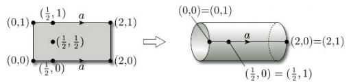
For each point x of the rectangle, we define the identification class of x to be the set of all points of the rectangle that are mapped to the same point of the cylinder as x is; for example, the class of (½, 0) consists of the pair of points (½, 0) and (½, 1), while the class of (½, ½) consists of just the point (½, ½). In general, we have the following definition:
Definition
Let f : X → Y be a function and let x ![]() X. The identification class of x, denoted by [x], is the set
X. The identification class of x, denoted by [x], is the set
Worked problem 5
Consider the identification of opposite edges of the rectangle [0, 3] × [0, 2] to form a torus, as illustrated in Figure 103.
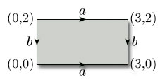
Write down the identification class [x] of each of the following points:

Solution
-
(a)

-
(b)
-
(c)
-
(d)
Problem 28
Consider the identification of opposite edges of the rectangle [0, 3] × [0, 2] to form a Klein bottle, as illustrated in Figure 104.
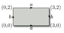
Write down the identification class [x] of each of the following points:

Answer
-
(a)

-
(b)

-
(c)
-
(d)

This now allows us to define the identification space of a polygon with edge identifications. In general the definition is as follows:
Definition
Given a topological space (X, T), a set Y, and a continuous function f : X → Y, the identification space I(X) of X under f is the set of all identification classes [x], for x ![]() X.
X.
Let X be a polygon with edge identifications and let Y be the object obtained by making those edge identifications. Let f be the map that creates Y from X, so that f(X) = Y. We now use this map to create a bijection F from I(X) to Y, by letting F : I(X) → Y map the identification class [x] to the image point f(x), that is, F([x]) = f(x). This function is clearly onto. To show that it is one-one, we must show that if F([a]) = F([b]), then [a] = [b]. This follows since, if F([a]) = F([b]), then f(a) = f(b), and thus [a] = [b]. Thus F is a bijection, as required.
The next step is to define a topology on I(X). We first note that there is an obvious map p from X onto I(X), sending each element x to its identification class [x]. We now define a subset U of I(X) to be open if p−1(U) is an open subset of X. This then creates the desired topology on I(X), as the following result demonstrates.
Theorem 15
Let (X, TX) be a topological space, let Y be a set, let f: X → Y be a function, let I(X) be the identification space of X under f and let [x] be the identification class of x ![]() X. Let p: X → I(X) be the function defined by p(x) = [x]. Then Tf = {U ⊆ I(X):p−1(U)
X. Let p: X → I(X) be the function defined by p(x) = [x]. Then Tf = {U ⊆ I(X):p−1(U) ![]() TX} is a topology on I(X).
TX} is a topology on I(X).
5.2.1 Proof
We check that Tf satisfies conditions (T1)–(T3) for a topology.
Since (T1)–(T3) are satisfied, Tf is a topology on I(X).
Thus (I(X),Tf) is a topological space. We give the topology Tf a special name.
Definition
The topology Tf defined in Theorem 15 is the identification topology for X under f.
We now use F to create a topology on Y = f(X). We define a subset U of Y to be open if F−1(U) is an open subset of X.
Recall that F([x]) = f(x).
Problem 29
Show that the family TY of open sets defined in this way comprises a topology on Y.
Answer
We check (T1)–(T3).
Since (T1)–(T3) are satisfied, TY is a topology on Y.
So we have a bijection F:I(X) → Y between the topological spaces (I(X),Tf) and (Y,TY). Furthermore, from the definitions of open sets in Tf and TY, we can deduce immediately that for each U ![]() TY, F−1(U)
TY, F−1(U) ![]() Tf and for each V
Tf and for each V ![]() Tf, F(V)
Tf, F(V) ![]() TY. Hence F is a homeomorphism between (I(X),Tf) and (Y,TY).
TY. Hence F is a homeomorphism between (I(X),Tf) and (Y,TY).
We have thus shown that the object created by identifying some or all of the edges of a polygon is a topological space homeomorphic to the identification space of the polygon. We now need to show that this topological space is Hausdorff and that every point has a disc-like or half-disc-like neighbourhood, to demonstrate that the space is indeed a surface.
5.3 Neighbourhoods
We know that a polygon X is a surface and so each point x in X has a disc-like or half-disc-like neighbourhood. We shall show that a map f that identifies edges of a polygon to create an object Y automatically creates corresponding disc-like or half-disc-like neighbourhoods of each point y = f(x) of Y.
If x is in the interior of X, there is no difficulty: the point x has a disc-like neighbourhood U which is mapped by f to a disc-like neighbourhood f(U) of y = f(x) in Y.
If x lies on the boundary of X, there are three cases to consider:
-
x lies on an edge that is identified with another edge, but not at a vertex of that edge;
-
x lies at a vertex of an edge that is identified with another edge;
-
x lies on a part of the boundary that is not identified with another part.
In each case, x has a half-disc-like neighbourhood in X. Some examples will help us determine which happens to these half-disc-like neighbourhoods after identification takes place.
5.3.1 Torus
If x lies on an edge, then each of the two points in [x] has a half-disc-like neighbourhood. When we identify edges, these neighbourhoods fit together to form disc-like neighbourhoods on the torus, as Figure 105 shows.
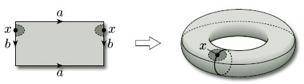
If x is a vertex, then each of the four points in [x] has a half-disc-like neighbourhood (in the shape of a quarter-disc). When we identify edges, these neighbourhoods fit together to form a disc-like neighbourhood on the torus, as Figure 106 shows.

5.3.2 Klein bottle
If x lies on an edge, then each of the two points in [x] has a half-disc-like neighbourhood (see Figure 107). When we identify edges, these neighbourhoods fit together to form disc-like neighbourhoods in the Klein bottle.
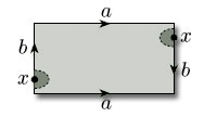
If x is a vertex, then each of the four points in [x] has a half-disc-like neighbourhood (as the shape of a quarter-disc – see Figure 108). When we identify edges, these neighbourhoods fit together to form a disc-like neighbourhood in the Klein bottle.
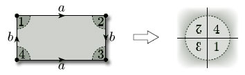
5.3.3 Torus with 1 hole
In our last example, we consider a pentagon with two pairs of edges identified. As we saw in Section 2.3, identification of the edges produces a torus with a hole. In this case there are five vertex-neighbourhoods to fit together, as shown in Figure 109. Identification of edges a and b shows that neighbourhoods 2, 3 and 4 fit together as shown. Identification of the edges b shows that neighbourhood 5 fits alongside neighbourhood 2, and identification of edges a shows that neighbourhood 1 fits alongside neighbourhood 4. However, neighbourhoods 1 and 5 do not fit together, and so we do not obtain a disc-like neighbourhood – rather we obtain a half-disc-like neighbourhood and the resulting vertex lies on the boundary of the hole.
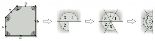
Finally consider a point x that lies on the edge c of the pentagon (see Figure 110). This has a half-disc-like neighbourhood. After identification of edges, this point lies on the boundary of the hole, and maintains its half-disc-like neighbourhood.
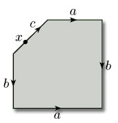
From these examples we can deduce that:
-
if a point lies on an edge that is identified with another edge, but not at a vertex of that edge, then after identification that point has a disc-like neighbourhood;
-
if a point lies on a part of the boundary that is not identified with another part, then after identification that point has a half-disc-like neighbourhood.
However, if a point is vertex of an edge that is identified with another edge, we have seen that after identification that point can have a disc-like or half-disc-like neighbourhood. We need to be sure that these are the only possibilities.
Consider the vertices x1, x2, …, xk of a polygon that are identified to the same point x by the edge identifications. In the polygon, each vertex xi has a half-disc-like neighbourhood that can be represented as in Figure 111. We shall call such a piece a wedge.

Some of the edges that come into each vertex xi are to be identified. Let us see what can happen. First, notice that the edge identifications that involve the vertices xi cannot have wedges that fit together to form two or more separate pieces: this is because, in such a case, the edge identifications would not identify all the vertices xi to a single point x. Also, because whole edges and not just vertices are identified, we cannot produce a situation such as that illustrated in Figure 112. Thus, the edge identifications that involve the vertices xi are such that all the wedges fit together to form a single neighbourhood. Either the point x is in the interior of the object so formed, as for the torus and Klein bottle, giving rise to a disc-like neighbourhood formed from the wedges, or the point x lies on the boundary, as for the torus with 1 hole. Thus:
-
if a point lies at a vertex of an edge that is identified with another edge, then after identification that point has a disc-like or half-disc-like neighbourhood.
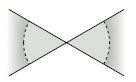
We have therefore demonstrated that every point of polygon with edge identifications has, after identification, a disc-like or half-disc-like neighbourhood. Furthermore, given any two points of the object obtained after identification, by choosing disc-like or half-disc-like neighbourhoods of sufficiently small radius, we can find neighbourhoods that do not intersect – so the object is Hausdorff. Combining these results with those of Section 5.2 tells us that an object formed by identifying edges of a polygon is a surface, as defined in Section 2.5. Furthermore, we know that such a surface is homeomorphic to the identification space of the polygon with edge identifications.
Conclusion
This free course provided an introduction to studying Mathematics. It took you through a series of exercises designed to develop your approach to study and learning at a distance and helped to improve your confidence as an independent learner.
Acknowledgements
Except for third party materials and otherwise stated (see terms and conditions). This content is made available under a Creative Commons Attribution-NonCommercial-ShareAlike 4.0 Licence
Course image: Alpha du centaure in Flickr made available under Creative Commons Attribution 2.0 Licence.
Don't miss out:
If reading this text has inspired you to learn more, you may be interested in joining the millions of people who discover our free learning resources and qualifications by visiting The Open University - www.open.edu/ openlearn/ free-courses