An introduction to minerals and rocks under the microscope
Use 'Print preview' to check the number of pages and printer settings.
Print functionality varies between browsers.
Printable page generated Friday, 19 April 2024, 11:25 AM
An introduction to minerals and rocks under the microscope
Introduction
The study of the structure and characteristics of minerals is fundamental to the identification of igneous, metamorphic and sedimentary rocks, and the interpretation of the environment in which they formed. This free course introduces the polarising microscope, the main tool used to study minerals in rock thin sections, which remains the foundation of learning to recognise, characterise and identify rocks.
The different atomic structures of minerals and their characteristics are explained, and the course develops the skills to identify minerals using features such as mineral shape, colour, grain size, opacity, refractive index and cleavage. The unique features of the polarising microscope are also covered, including extinction, birefringence and pleochroism.
Recognising minerals and understanding their structure is the basis for recognising rocks and interpreting microtextures to learn how they were formed. Evidence gathered by careful study of minerals in thin sections is a key part of the interpretation of igneous, metamorphic and sedimentary rocks.
If you'd like an interactive overview of the geological makeup of the landscape of the British Isles, take a look at our Geology Toolkit.
This OpenLearn course provides a sample of level 2 study in Science.
Learning outcomes
After studying this course, you should be able to:
understand the facts, concepts, principles, theories, classification systems and language associated with minerals and rocks
use the essential terms, concepts and strategies of mineralogy
apply knowledge and understanding of the study of rock thin sections using a polarising microscope
work with and recognise a variety of minerals and microtextures in igneous, metamorphic and sedimentary rocks
make systematic descriptions and identifications of minerals in rocks, observing them using images of thin sections viewed under a polarising microscope, and deduce how and in what environments the minerals and rocks were formed.
1 Minerals and the crystalline state
1.1 Introduction
Rocks are made of minerals and, as minerals are natural crystals, the geological world is mostly a crystalline world. Many large-scale geological processes, such as the movement of continents and the metamorphism of large volumes of rock during mountain building, represent the culmination of microscopic processes occurring inside minerals. An understanding of mineral structures and properties allows us to answer questions such as, 'Why is quartz so hard?' and 'Why is quartz so often the dominant type of sand grain on a beach?' and 'How can solid rocks bend into huge folds, or flow like a liquid over geological time?' Minerals and rocks are also, of course, natural resources that provide the inorganic raw materials for almost everything humans use. A good scientific understanding of their origins, occurrence and properties helps to maximise their potential benefits to humanity. In this course, you will look at mineral and rock specimens in various ways (Box 1).
Box 1 Mineral and rock specimens in the Digital Kit and Virtual Microscope
In this course, we will often refer to mineral specimens and rock specimens in the Digital Kit and the Virtual Microscope. You may find it easier to open them in separate tabs in your browser, which you can do by holding down the 'Ctrl' button before left-clicking on the link with your mouse (or equivalent for non-mouse users). To get back to this course please press the back button in your browser.
Activity 1.1 Introduction to the Digital Kit
Task 1
This activity is designed to familiarise you with the operation and content of the Digital Kit, which provides access to images and information about the mineral and rock specimens used in this course.
Open the Digital Kit and you should see a screen similar to the one shown in Figure 1. We will use the mineral galena to illustrate the Digital Kit, but this may not be the image that appears the first time you access the Digital Kit.
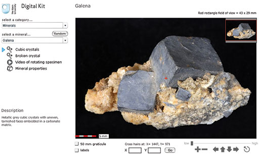
The screen is divided into the field of view of the specimen and several functional areas that control the images, including a main viewing window, zooming and panning facilities, and buttons/hyperlinks to other images, video clips and mineral properties.
In the upper left-hand corner, the catalogue of specimens can be accessed via two drop-down menus. Click the upper menu to select from the categories of minerals, rocks or fossils. Select 'Minerals' for this demonstration.

The lower drop-down menu lists different minerals in alphabetical order. Select 'Galena' from the menu.
A very useful feature of the Digital Kit is a 'Random' button (adjacent to the catalogue), which can be used for self-test and revision purposes. When clicked, a random mineral, rock or fossil is presented, depending on which of these three categories is already selected. There are two stages of working in random mode: clicking the 'Clue' button gives the description (at the bottom of the left-hand column), and clicking 'Reveal' gives the name as well.
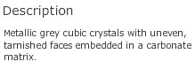
Once the specimen (galena, in this case) has been selected, a series of buttons and a description of the mineral appear below the two drop-down menus, as shown here for galena. Several views and, in most cases, a video clip of a rotating image are available for each specimen (see below). Finally, a mineral properties page is given for each mineral.
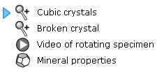
For this demonstration, select the 'Cubic crystals' view.
- A short description of each specimen appears below the menus.
The main window shows the full specimen view when initially selected from the menu. At the centre of the field of view (at any magnification) is a small cross. As explained below, the coordinates of this cross are given, allowing specific points in the image to be identified.
The image can be manipulated either by zooming in and out, or by panning around the specimen at different magnifications. As the main image is zoomed or panned, the inset image in the top right-hand corner shows its location as a red rectangle. The dimensions of the field of view displayed are given in millimetres in the top right above the viewing window.
The image can be moved in several different ways, by:
- clicking and dragging the image itself
- using the arrows on the right below the viewing window (further explained below)
- clicking and dragging the red rectangle in the inset image
- clicking and holding down the arrow keys on the keyboard you are using.
The image magnification can be varied by zooming in and out of the field of view. This can be achieved in various ways:
- A set of image manipulation controls on the right below the viewing window contains all the zooming and panning functions. These are explained in point 5, below.
- If you wish to zoom into a specific point on the image, simply click on it and it then becomes the new centre of the image at a higher magnification. Another click zooms in further.
- Zooming in and out can also be achieved using the computer keyboard. Press the 'A' key to zoom in, and the 'Z' key to zoom out.
A 5 mm scale bar at the bottom left-hand corner of the viewing window shows millimetre increments.
Below the viewing window on the right-hand side are a series of image manipulation controls. Click on the '+' to zoom in, and the '−' to zoom out. Click on one of the four arrows to move the viewing window across the image in the direction indicated. The circle containing an arrow resets the window to the full specimen view. Above the controls, a magnification slide bar indicates the zoom level. The magnification slider can be clicked (it will go black as the mouse passes over it) and dragged to the right and left to zoom in and out of the specimen. You will find this very useful.

We recommend that you try all the ways of moving an image and changing its magnification, to see which are best for you.
Below the viewing window on the left-hand side are two tick boxes.

When the '50 mm graticule' box is selected, a 50 mm graticule is superimposed over the image, allowing direct measurement of features anywhere on a specimen once the features are moved to the centre of the field of view. Clicking on either of the two curved arrows rotates the graticule to enable features to be measured in any orientation.
When the 'labels' box is selected, labels are superimposed on the specimen, identifying particular features. These labels are shown only at the lowest magnification. If the 'labels' box is clicked when at a higher magnification, the image reverts to the lowest magnification and the labels are shown.
The location of the small central cross (the 'cross hairs') is constantly displayed below the viewing window as X and Y coordinates. The sample can be moved to a specific location by typing its X and Y coordinates into the boxes and clicking the 'Go' button. This useful feature allows locations of particular features to be communicated between different users.

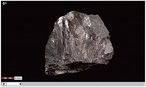
When a 'Video of rotating specimen' button is selected (a right-pointing arrowhead in a circle), a video clip window replaces the zooming and panning window.
After the video clip window is launched, a dark-grey fill extends across the bar below the image, indicating that the clip is loading into the computer's memory. The button at the bottom left starts (or pauses) the video clip. A particular position in a rotation video clip can be specified using the number of degrees shown at the top left (e.g. 60°) of the video clip window.
- Finally, when the 'Mineral properties' button is clicked, a range of mineral properties is displayed.

| Crystal system | cubic |
| Formula | PbS |
| Colour | dark grey to grey-black |
| Lustre | metallic to dull |
| Form | cubes and octahedra; also massive, granular |
| Cleavage | 3 perfect cubic |
| Fracture | subconchoidal |
| Hardness | 2.5 |
| Relative density | 7.6 |
| Types | |
| Common occurrence | hydrothermal vein |
| Comments | opaque; colour, form, density, cleavage and lustre can be diagnostic |
Now answer the following questions to help you find your way around the Digital Kit.
Question 1.1.1
In the Digital Kit select 'Galena' and 'Broken crystal'. Zoom in on the specimen and pan around to explore the features on the broken surface. How many cleavage orientations does galena exhibit? Look at the video clip of the rotating galena specimen, which will help you to perceive the cleavages more easily in three dimensions. Confirm your answer by selecting 'Mineral properties'.
Question 1.1.2
- a.Go to 'Quartz' and select 'Variety amethyst'. How long is the amethyst crystal on the far left? Measure it using the graticule.
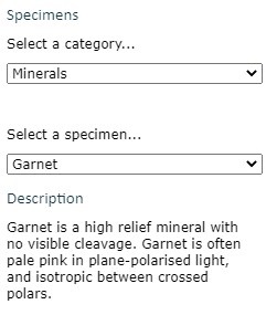
- b.Go to 'Garnet' and select 'Red crystals in gneiss'. Go to coordinates X = 1860, Y = 930. Is any red garnet visible at the point denoted by the cross hairs?
Answer
- a.It is about 16 mm. Note that there are large divisions on the graticule every 10 mm.
- b.No, garnet is not visible at this point, only a white mineral is visible at the stated coordinates.
Question 1.1.3
- a.Which of the following minerals has the highest density and which the lowest density: garnet, gypsum and quartz?
- b.Which of the following minerals is the hardest, and which is the softest: galena, hematite and pyrite?
- c.Supply the missing words in the following statements.
- i.Selenite is a variety of the mineral ___________
- ii.The mineral ___________ may have a form described as 'kidney-shaped'.
- iii.Chert is a variety of the mineral ___________
- iv.Pure pyrite contains ___________chemical elements.
Answer
- a.Garnet has the highest density (3.6-4.3); gypsum has the lowest density (2.3). Quartz is in between (2.65). (Density values quoted are relative to water.)
- b.Pyrite is the hardest (6-6.5), galena the softest (2.5). Hematite has hardness 5-6.
c.
- i.Selenite is a variety of the mineral gypsum.
- ii.The mineral hematite may have a form described as 'kidney-shaped'.
- iii.Chert is a variety of the mineral quartz.
- iv.Pure pyrite contains two chemical elements. (These are iron and sulfur.)
Take a look at the granite in Figure 2a and examine the granite rock specimen in the Digital Kit. This rock is composed of three distinct types of crystal, each of which is a different mineral: shiny black biotite mica (cf. Digital Kit); cloudy orthoclase feldspar (cf. Digital Kit); translucent grey quartz (cf. Digital Kit).
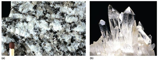
The junction between any two adjacent crystals in the rock is called a grain boundary. Grain boundaries occur where crystals develop in contact with each other - here, during the cooling and crystallisation of magma to form granite. Grain boundaries also develop when minerals grow in the solid state during metamorphism. Where the crystals form an interlocking mass, as in granite or marble, they rarely have the opportunity to develop good crystal faces. By contrast, the best-formed crystals are often ones that have grown into cracks or cavities (such as a gas bubble in a lava flow). Figure 2b shows several such quartz crystals that have grown into a cavity.
Crystals may be objects of great beauty, in part because of their almost perfectly flat crystal faces and geometric shapes. This regular external appearance is caused by a highly ordered internal arrangement of atoms, known as the crystal structure, which leads to distinct (and to some extent predictable) physical and chemical properties.
Minerals, by definition, are solid substances. Before looking at the crystalline world in more detail, the next section considers briefly the various physical states that matter can have, and the transition from one state to another - concepts that remain relevant at various stages throughout the course.
1.2 States of matter
Substances generally exist in one of three different states: as a gas, liquid or solid. Figure 3 illustrates these states in terms of their atomic arrangements. Atoms or molecules in a gas move at high velocities, and the distances between them are large, so gases have low densities. In a liquid, the atomic motions are slower, and the atoms are closer together (producing a higher density). If you could take a snapshot of the atoms in a liquid or a gas, you would see a random or disordered arrangement. Another snapshot, taken a fraction of a second later, would look different. So, the internal structures of liquids and gases are disordered both in space and time.
A kind of real-life snapshot of a liquid structure can be taken by very rapidly cooling the liquid to quench it, so that it solidifies before the atoms have had time to rearrange themselves. At low temperatures, there is not enough thermal energy for the atoms to move relative to each other. The quenched material is a disordered solid, known as an amorphous solid or glass (Figure 3).
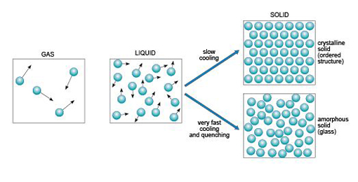
By contrast, slow cooling of a liquid allows atoms to arrange themselves into an ordered pattern, which may extend over a huge number of atoms. This kind of solid is called crystalline. So if a melt of a given composition (e.g. SiO2) is cooled very rapidly it will produce a silica glass, whereas if it were cooled slowly it would produce a crystalline solid composed of quartz crystals.
It is important to note that compared with crystalline solids, glass is not a particularly stable form of matter. Over many years, glass may slowly convert into a crystalline form in a process called devitrification, and this can sometimes be observed in centuries-old window panes, where circular frosted patches of tiny crystals have formed within the glass.
The states in which a single substance can exist - gas, liquid or solid - are referred to as phases of matter. The range of pressures and temperatures over which a particular phase is stable (i.e. its stability field) can be shown on a phase diagram. The stability fields of different phases may be represented as areas separated by boundary lines on a pressure-temperature diagram, as illustrated in Figure 4, a phase diagram for H2O. A change of temperature (or pressure) may result in a phase transformation; for example, liquid H2O (water) can be heated to form a gas (steam), or cooled to form a solid (ice).

At the surface of the Earth, with a typical pressure of one atmosphere (approximately 105 Pa), a crystalline solid, ice, is the stable phase of H2O at temperatures below 0 °C. Above this temperature (the melting point of ice), solid ice transforms to liquid water. The boundary between the solid and liquid stability fields is a phase boundary, and is indicated by a solid line in Figure 4. If the temperature continues to increase at constant pressure (along the horizontal dashed line in Figure 4), the phase boundary between the liquid (water) stability field and the gas (steam) stability field is reached. This boundary represents the boiling temperature of water. Although only the effect of changing temperature has been considered so far, it is important to note that both the melting temperature and the boiling temperature vary with pressure. The point where all three phase boundaries for H2O meet is called the triple point, a unique pressure and temperature where solid (ice), gas (steam) and liquid (water) can coexist.
-
How would the boiling temperature of water, measured at the top of a high mountain where the atmospheric pressure is much lower, compare with its boiling temperature at sea level?
-
The H2O phase diagram (Figure 4) shows that the boiling temperature of water (indicated by the liquid/gas phase boundary) decreases with decreasing pressure. Thus, on top of a mountain, where atmospheric pressure is lower, water boils at a lower temperature.
1.3 Physical properties of minerals in hand specimen
Physical properties, such as colour and density, are those that can be observed without causing any change in the chemical composition of a specimen, whereas chemical properties determine how a substance behaves in a chemical reaction. Many of the physical properties of minerals can be predicted from a detailed knowledge of their crystal structures, which can be obtained by various analytical techniques. Alternatively, physical properties can be used to infer particular aspects of a mineral's internal structure.
Several physical properties of minerals can be readily observed from hand specimens, and can be used for recognising and distinguishing different minerals.
1.3.1 Crystal shape
Well-developed crystals show a number of flat faces and a distinct shape. The shape of the crystal, and the precise arrangement of its crystal faces, relate to its internal structure, and are expressions of the regular way the atoms are arranged.
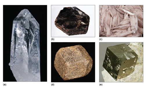
Many terms are used to describe the shapes of different crystals. These can be broadly grouped into three categories:
- prismatic (the crystal is stretched out in one direction; Figure 5a)
- tabular (the crystal is squashed along one direction, so appears slab-like or platy; Figure 5b and c)
- equidimensional (the crystal has a rather similar appearance in different directions, e.g. cubes, octahedra, and 'rounded' crystals with many faces of similar size; Figure 5d and e).
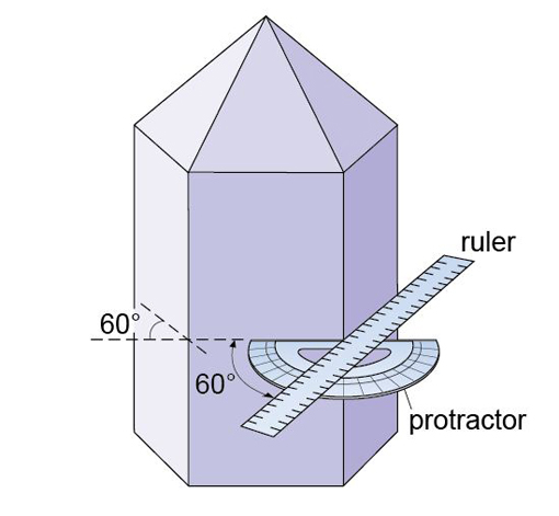
Crystals of the same mineral tend to show the same general crystal shape. Quartz, for example, is almost always prismatic, rather than tabular or equidimensional. However, the exact shape of crystals of the same mineral can vary, depending on the conditions at the time of growth. Two crystals of the same mineral may differ in the relative sizes of specified crystal faces, or some faces may not be present. Although the relative sizes of specific crystal faces often vary, the angles between such faces are always fixed as they are defined by the crystal structure. This consistency of angles may be verified by measuring the angle between crystal faces with, for example, a protractor (Figure 6) or a more accurate device called a goniometer.
-
Some minerals have a crystal shape that is best described as 'acicular' (i.e. needle-like). In which of the three general categories of crystal shape mentioned above do acicular crystals lie?
-
Acicular crystals belong to the prismatic category as they are stretched out in one direction.
Note that there is often a distinction between the shape of individual crystals and the form they may take when many crystals are assembled into an aggregate. For example, some minerals have acicular crystals that radiate in all directions away from a central point, forming a globular (i.e. spherical) aggregate. Aggregates may also be fibrous, columnar, dendritic (clusters of crystals in fern-like branches), and so on. When crystals grow together in a solid mass, in which individual crystals cannot clearly be seen, aggregates are described as massive.
1.3.2 Colour
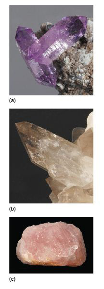
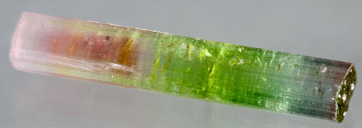
The colour of a mineral can be its most obvious feature, but colour can also be one of the least reliable properties for identifying minerals. Many minerals show a wide range of coloration, often caused by tiny amounts of impurities. For example, pure quartz (SiO2) is colourless; minute quantities of Fe3+ iron induce a purple coloration, characteristic of the variety of quartz known as amethyst (Figure 7a). Small amounts of aluminium cause the dark coloration of smoky quartz when the crystal has been exposed to natural radioactivity (Figure 7b). The reason for the pink colour in rose quartz (Figure 7c) is not fully understood; titanium or manganese may be involved, as may minute fibrous crystals of a complex mineral within the quartz. The yellow colour of citrine (another quartz variety) is probably due to minute amounts of iron hydrates dispersed within the crystal. (Many examples of citrine for sale are actually artificially heated or irradiated amethyst.) Milky quartz is white and cloudy as a result of tiny bubbles of fluid (liquid and/or gas). In a few minerals, such as tourmaline, an individual crystal may be multicoloured (Figure 8), reflecting subtle changes in chemical composition as it grew.
Some minerals do, however, have reliable and distinctive colours. Silicate minerals that contain large amounts of iron are typically dark green or black. These minerals, which often also contain magnesium, are called ferromagnesian minerals; they include olivine, pyroxene, amphibole and biotite mica (see Section 3).
1.3.3 Lustre
The term 'lustre' refers to the surface appearance of a mineral, which depends on the way it reflects light. Typical terms used to describe a mineral's lustre include vitreous (rather like glass), metallic and resinous. Quartz (Figure 5a) has a vitreous lustre, as do many other silicate minerals, such as feldspar. When transparent, like window glass or clear coloured glass, the term 'glassy' lustre may be used instead of vitreous: quartz, for example, often has a glassy lustre.
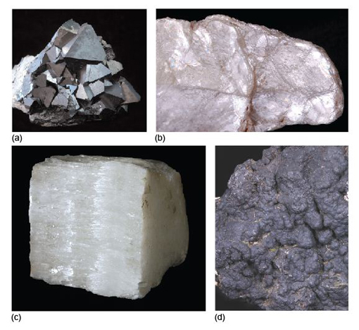
Some opaque minerals scatter light very strongly, giving rise to shiny, reflective surfaces and a metallic lustre, such as seen in pyrite, galena (both available in the Digital Kit) and magnetite (Figure 9a). Other examples are pearly lustre (looking like pearls) (Figure 9b), silky lustre (like shiny threads or fibres) (Figure 9c), and a dull or earthy lustre (Figure 9d). Note that, as in the case of gypsum (Figures 9b and c), different varieties of the same mineral may show different types of lustre.
1.3.4 Cleavage
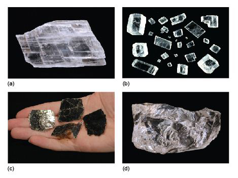
If a crystal is struck with a hammer, it will probably shatter into many pieces. Some minerals, such as calcite (cf. Digital Kit), break into well-defined blocky shapes with flat surfaces. These are called cleavage fragments (Figure 10a and b) and the flat surfaces are called cleavage planes. Note that cleavage planes, which occur within a crystal, are not the same as crystal faces.
Cleavage arises when the crystal structure contains repeated parallel planes of weakness (due to weak chemical bonds), along which the crystal will preferentially break. The mineral mica (which includes biotite and muscovite (cf. Digital Kit)) has such perfect cleavage in one direction that it can be readily split, or cleaved, into wafer-thin sheets (Figure 10c), using just a fingernail. Some minerals break into irregular fragments that lack flat surfaces (except for any remnants of original crystal faces). In the case of quartz (Figure 10d and Digital Kit), which has no cleavage, the broken pieces have a curved fracture pattern, called conchoidal (pronounced 'con-koi-dal') fracture. Some minerals have only one set of cleavage planes, others have two sets, and a few (such as calcite) have three. In minerals with only one or two sets of cleavage planes, some broken surfaces will show just fracture.
1.3.5 Density
Density is a measure of how heavy an object is for a given volume. You can get a general idea of the relative densities of different minerals just by picking them up: a piece of galena feels heavier than a piece of quartz of the same size. The density of a mineral depends on its chemical composition, the type of bonding and its crystal structure. The standard unit of density is kg m−3. Examples of the relative densities of various minerals compared with water at room temperature (about 1000 kg m−3) are shown in Table 1. The relationship between density and crystal structure is explored further in Section 1.4.
| Mineral | Symbol/formula | Relative density at room conditions (compared with water = 1.0) |
|---|---|---|
| graphite | C | 2.2 |
| quartz | SiO2 | 2.7 |
| diamond | C | 3.5 |
| barite | BaSO4 | 4.5 |
| galena | PbS | 7.6 |
| silver | Ag | 10.5 |
| gold | Au | 19.3 |
1.3.6 Hardness
Hardness is loosely defined as the resistance of a material to scratching or indentation. The absolute hardness of a material can be determined precisely, using a mechanical instrument to measure the indentation of a special probe into a crystal surface. However, you can get a general idea of a mineral's relative hardness, by undertaking a few simple scratch tests.

The 19th century German mineralogist, Friedrich Mohs, devised a useful scale of mineral hardnesses, consisting of well-known minerals, ranked in order of increasing hardness, from talc, with a hardness of 1, to diamond, with a hardness of 10 (Table 2). Compared with an absolute hardness scale, Mohs' scale is highly non-linear (diamond is about four times harder than corundum; Figure 11c and b) but, because the scale uses common minerals, it provides a quick and easy reference for geologists in the field. Minerals with a hardness of less than 2.5 may be scratched by a fingernail, whereas those with a hardness of less than 3.5 may be scratched by a copper coin, and so on.
| Mohs' hardness | Reference mineral | Non-mineral example (hardness in brackets) |
|---|---|---|
| 1 | talc | |
| 2 | gypsum | |
| fingernail (2.5) | ||
| 3 | calcite | |
| copper coin Footnotes 1 (3.5) | ||
| 4 | fluorite | |
| 5 | apatite | |
| window glass/ordinary knife blade (5.5) | ||
| 6 | orthoclase feldspar Footnotes 2 | |
| hardened steel (6.5) | ||
| 7 | quartz | |
| 8 | topaz | |
| 9 | corundum | |
| 10 | diamond |
Footnotes
Footnotes 1 Note that many of today's 'copper coins' are copper-plated steel and are harder below the copper coating. Back to main textFootnotes
Footnotes 2 Other types of feldspar may have a slightly greater hardness, between 6 and 6.5. Back to main text-
Will quartz scratch topaz (Figure 11a)?
-
The hardness of quartz is 7, whereas topaz has a hardness of 8, so topaz will scratch quartz but not the other way round.
Hardness should not be confused with toughness, which is the resistance of a material to breaking. Many minerals are hard, but they may not be tough. Diamond, for example, is the hardest known material, but it is not tough: it will shatter if dropped onto a hard surface.
1.4 The atomic structure of crystals
The atomic structure of a mineral influences many of its physical and optical properties. This section briefly considers some of the main ways in which atoms are arranged, and how they are bonded, starting with metals, which have some of the simplest atomic arrangements possible. Variations on these arrangements provide the structural foundations of many common minerals.
1.4.1 Metallic structures and bonding
Metal crystals are built from layers of densely packed metal cations (atoms that have lost one or more electrons, leaving them positively charged). The ions are organised in regular, close-packed arrangements. In close-packing, a layer of identically sized atoms (or ions) occupies the minimum possible space - like a raft of hard spheres (e.g. marbles) in contact with each other. Each atom has six neighbours in a plane. The three-dimensional structure of a metal involves the successive stacking of close-packed layers on top of each other.
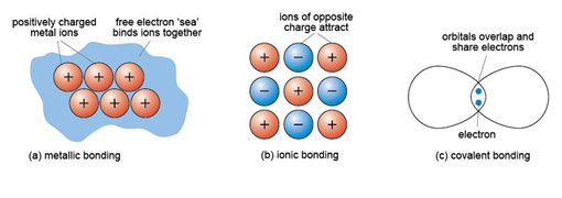
In metallic bonding, atoms donate one or more outer electrons to a free electron 'sea' (Figure 12a), which flows between and around the cations and acts as a kind of glue, holding them together. This kind of bonding is uniform in all directions, so that metallic structures are dense and close-packed. The electron mobility renders metals both malleable and ductile, which are vital properties for producing thin sheets and for stretching out to form thin cables or filaments (e.g. copper wire).
1.4.2 Ionic structures and bonding
About 90% of all minerals are essentially ionic compounds. An ionic bond is generated by the transfer of one or more electrons from one atom to another. This creates two ions of opposite charge, which are attracted to each other (Figure 12b). For example, in halite (sodium chloride, NaCl) there is a positively charged sodium cation, Na+, and a negatively charged chlorine anion, Cl−. As with metallic bonding, ionic bonds are non-directional, so ionic crystals tend to have fairly dense, close-packed structures. However, ionic bonds tend to be stronger than metallic bonds, so crystals containing ionic bonds tend to be unmalleable and much more brittle than metal crystals.
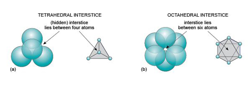
Even though a close-packed structure looks densely packed, there are actually lots of spaces between the atoms. These spaces are called interstices and are important in metallic structures because they provide sites for smaller atoms to reside. Interstices also provide a basis for many ionic structures: they provide locations for smaller ions, in the presence of large ions. There are two kinds of interstices: a tetrahedral interstice, surrounded by four atoms, one at each of the corners of an imaginary tetrahedron (Figure 13a); and an octahedral interstice, surrounded by six atoms, arranged at the corners of an imaginary octahedron (Figure 13b).
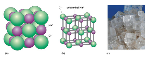
The mineral halite (Figure 14) is an example of a structure with octahedral interstices (as in Figure 13b). The chlorine ions are arranged a bit like the atoms in a metal - although they do not quite touch each other. The sodium ions, which are much smaller, fit snugly between the large chlorine ions, as illustrated in a space-filling model (Figure 14a).
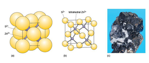
The structure of sphalerite (zinc sulfide, ZnS) (Figure 15) has a close-packed arrangement of sulfur ions, a structure in which zinc ions fill half of the tetrahedral interstices (as in Figure 13a).
1.4.3 Covalent structures and bonding
A covalent bond is formed when two atoms share two electrons, through overlap and merging of two electron orbitals, one from each atom (Figure 12c). Crystals containing covalent bonds tend to have more complex structures than those of ionic or metallic structures. Covalent bonding requires the precise overlap of electron orbitals, so if an atom forms several covalent bonds, these are usually constrained to specific directions. As covalent bonds are directional, unlike metallic or ionic bonds, this places additional constraints on the arrangements of atoms within such a crystal. One result is that covalent structures tend to be more open - and hence have lower densities than metallic or ionic structures.
Diamond is an example of a covalently bonded solid. In this form of carbon, each atom is covalently bonded to four other carbon atoms, arranged at the corners of a tetrahedron (Figure 16a). The resulting structure, which has a repeating cubic shape, is illustrated in Figure 16b. The structure contains much more unoccupied space than close-packed metal structures.
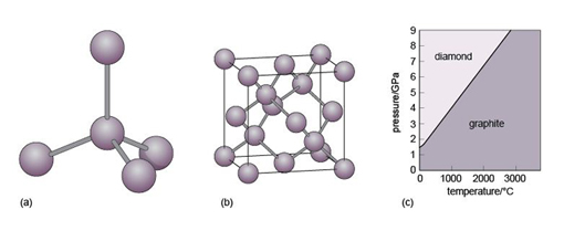
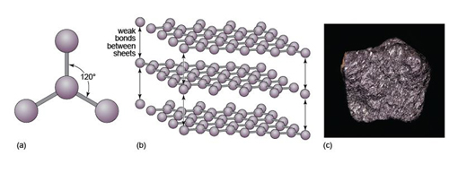
Another form of solid carbon with covalent bonding is graphite. Unlike those in diamond, the carbon atoms in graphite are covalently bonded to three neighbours in the same plane (Figure 17a), producing a strong sheet of carbon atoms. However, each carbon atom has one extra electron available for bonding that forms very weak bonds, which serve to keep the carbon sheets together (Figure 17b).
-
How do the crystal structures of diamond and graphite account for the differences in hardness between the two minerals?
-
Diamond has a three-dimensional bonding pattern, with identical bonding in all directions, and no 'weak' directions. Graphite has a mainly two-dimensional pattern, with sheets of C-C bonds. Bonds between the sheets are very weak, so sheets can easily slide past each other, explaining graphite's use as a lubricant and why it is soft enough to mark paper.
Diamond and graphite have the same chemical composition (pure carbon) but different crystal structures. They are known as polymorphs of carbon. Diamond is formed under higher pressures than graphite (Figure 16c), and is less stable than graphite at the surface of the Earth. However, because of the strong bonding, it is very difficult to break down the diamond structure, so diamonds (fortunately) will not spontaneously transform into graphite! Note that not only is diamond harder than graphite, but it is also denser, as predicted by its structure (Table 3).
| Substance | Relative density at room conditions(compared with water = 1.0) | Structure and bonding |
|---|---|---|
| ice, H2O | 0.9 | open structure; covalent bonds plus weak bonds between H2O molecules |
| graphite, C | 2.2 | open structure; covalent bonds plus weak bonds between layers |
| feldspar, KAlSi3O8 | 2.5 | open structure; predominantly covalent bonds |
| quartz, SiO2 | 2.7 | open structure; predominantly covalent bonds |
| olivine, Mg2SiO4-Fe2SiO4 | 3.2-4.4 | structure based on close-packing, but with ionic and covalent bonds. Density increases as Fe content increases |
| diamond, C | 3.5 | structure based on close-packing, but with covalent bonds |
| barite, BaSO4 | 4.5 | ionic bonds between barium and sulfate groups |
| hematite (iron oxide), Fe2O3 | 5.3 | structure based on close-packing; ionic and metallic bonds |
| galena (lead sulfide), PbS | 7.6 | structure based on close-packing; ionic and metallic bonds |
| silver, Ag | 10.5 | close-packed structure; metallic bonds |
| gold, Au | 19.3 | close-packed structure; metallic bonds |
Minerals are never chemically pure; they always contain some foreign atoms. These impurity atoms may simply squeeze into the interstices. Another possibility is that certain elements may be able to directly replace (substitute for) the normal atoms in the ideal structure - although, for a comfortable fit, the substituting element must have a similar size and charge to the original atom. This phenomenon is called ionic substitution. An example is the substitution of Fe2+ for Mg2+, or Mg2+ for Fe2+, which occurs in the mineral olivine (Section 3.3.1).
1.5 Crystal defects and twinning
Virtually all crystals contain minute imperfections or defects. The effect of defects on the physical and chemical properties of a crystal can be out of all proportion to their size. Defects come in several types. Point defects may involve missing or displaced atoms in the crystal structure, giving empty sites, or vacancies. Such defects make it much easier for atoms to diffuse through the crystal structure, by moving between vacant sites. This is important because the rate of diffusion of atoms through a crystal lattice can determine the speed at which processes such as weathering, or other chemical reactions (e.g. during metamorphism), will proceed.
Minerals in deformed rocks, such as those from mountain belts, contain large numbers of line defects caused by rows of atoms that are out of place in the crystal structure. Figure 18 shows an artificial example. Such defects affect the mechanical strength of a crystal, which determines the strength of rocks and how they deform under intense pressure. During deformation, progressive movement along flaws in crystals takes place in tiny steps, as bonds are broken and re-formed.
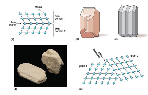
A third type of defect is called a planar defect. Crystals grow by the progressive addition of atoms onto a surface. 'Mistakes' in the stacking of new planes with respect to previously formed planes are common during crystal growth. These planar defects can have a profound effect on the way atoms are stacked, and can produce distinct regions called domains within a single crystal. One such planar defect is a boundary that separates two domains of a crystal that are mirror images (Figure 19a). The result is called a twinned crystal. Various types of crystal twinning exist, and in each case a single crystal consists of two or more regions in which the crystal lattice is differently orientated. The different regions of the twinned crystal may be related in various ways, such as by reflection in a mirror plane or by rotation about a symmetry axis (see Section 1.6). Twinning is especially common in feldspar. Orthoclase feldspar often displays simple twinning, in which the crystal is divided into two domains with a different structural orientation (Figure 19b and d). Other types of feldspar (e.g. plagioclase feldspar) may have a more complex type of twinning, called multiple twinning, in which a single crystal has many different domains (Figure 19c).
1.6 Crystal symmetry and shape
In this section, you will investigate the relationship between the shape and symmetry of crystals, consider why minerals have only a limited number of crystal shapes, and discover how the shape of a mineral relates to its internal structure.
1.6.1 Crystal symmetry
When you first look at a collection of minerals in a museum, there may seem to be an infinite variety of crystal shapes. However, on closer inspection there is an underlying order, and this is best seen by the consistency in the angles between crystal faces for particular groups of minerals. Crystals possess a variety of symmetries, and it has been demonstrated by X-ray methods that symmetry visible in hand specimen relates to the internal arrangement of atoms.
Most people have an idea of what is meant by symmetry, as many everyday objects and living things possess it. There are two main types of symmetry:
- reflection symmetry where one side of an object is the mirror image of the other side (e.g. insects, birds and spoons)
- rotational symmetry where an object looks the same after a certain amount of rotation (e.g. many flowers, starfish and bicycle wheels).
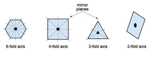
Many complicated patterns such as carpet or wallpaper designs have symmetry, but these can sometimes be a little difficult to discern. Consider, for example, an object with obvious symmetry, such as a snowflake (Figure 20). Each snowflake can be rotated by 60º about an axis perpendicular to the page and it will look exactly the same as it did before. The operation can be repeated six times in a full 360º rotation of the page, and at each 60º interval the snowflake will look the same. Thus the snowflake has a six-fold rotational symmetry. A snowflake also possesses reflection symmetry; if you 'split' the snowflakes along certain planes, called mirror planes, the two halves are mirror images of each other. Some examples of rotational and reflection symmetry found in crystals are illustrated in Figure 21.

1.6.2 Crystal lattices and unit cells
A typical crystal contains billions of atoms in a highly ordered structural arrangement. Perhaps surprisingly, the essence of such a complex structure can be described relatively simply. How is this possible?
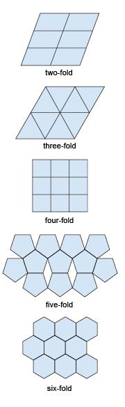
If you tried to tile a two-dimensional area such as a bathroom floor without any gaps, you would do this by adding tiles that fitted together. In fact, only tiles with two-, three- four- and six-fold symmetry allow for successful tiling (Figure 22). Similarly, if you tried to produce a three-dimensional structure (like a crystal) without any gaps it would require the repetition of building blocks (i.e. 3D repeating units) with particular shapes. As with two-dimensional tiling, the only kinds of rotational symmetry axis possible in three-dimensional crystals are two-, three-, four- and six-fold axes.
A lattice is an array of objects or points that form a periodically repeating pattern in two or three dimensions. In a crystal lattice, the repeating pattern is simply an arrangement of atoms (or ions) that is located at regular points, called lattice points.
Figure 23a shows a three-dimensional lattice, the building of which can be envisaged by simply stacking a series of identical two-dimensional lattices on top of each other. A crystal is, in effect, a structure formed by countless numbers of identical tiny building blocks, called unit cells (Figure 23b), and these make up the crystal lattice. Each mineral has a specific unit cell, which is defined according to the lengths of its sides and their angular relationships. Each unit cell contains one or more different kinds of atoms joined to each other by chemical bonds. Shapes of unit cells vary from one mineral to another; all have six sides (three sets of parallel faces, though not necessarily perpendicular to each other).
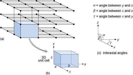
To define the resulting three-dimensional lattice, it is convenient to specify reference directions, x, y and z, which are chosen to be parallel to three edges of the unit cell (Figure 23b). These are known as crystallographic axes, and it is important to realise that they are not always at 90° to each other. The angles between the axes are denoted by the Greek letters α, β and γ (alpha, beta and gamma), as shown in Figure 23c. The size of the unit cell is given by the lengths of the three edges, a, b and c, as shown in Figure 23b. The unit cell is extremely small - typically less than 1 nm (10−9 m) in any direction. It is therefore a huge jump in scale from a single unit cell to a single crystal visible to the naked eye. With an edge length of 1 nm, a crystal only 1 mm3 requires 1018 unit cells to build it: a vast number.
A three-dimensional lattice (which may have billions of lattice points) can be represented by just six numbers: the lattice parameters a, b, c, α, β and γ. In the next section, you will see how the shape of the unit cell relates to a crystal's symmetry, and what this means for the external shapes of crystals.
1.6.3 Crystal systems
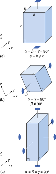
Most three-dimensional lattices display some symmetry, although the symmetry elements (e.g. rotation axes and mirror planes) can be in any direction. Some arrangements of symmetry elements place special constraints on the shape of the unit cell. For example, a four-fold rotation axis requires the unit cell to have a square section at right angles to the symmetry axis (Figure 24a). Three four-fold axes at right angles to each other imply that the unit cell must be a cube, and so on.
Crystals are classified on the basis of this three-dimensional symmetry (and hence the shapes of their unit cells) into one of seven different crystal systems (Figure 25).
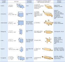
The beauty of crystallography is that you do not need to see the lattice, the unit cell, or the atoms in order to deduce this symmetry. The extent of symmetry varies from the cubic system, which has the most symmetry, to triclinic, which has the least. Generally, the more symmetry a crystal has, the more constraints this places on its external shape. Crystals belonging to the cubic system tend to have equidimensional shapes, such as cubes, octahedra (with eight faces), or rather rounded-looking crystals with many faces (e.g. dodecahedra, with twelve faces). Pyrite and galena, for example, can have very simple cube-shaped crystals, which clearly indicate their underlying cubic symmetry. These same minerals may also have more complex shapes, with many more faces, but each shape still has the symmetry that places the mineral within the cubic system. The same possibility for variation within certain limits applies to other minerals in different crystal systems. Despite their complexity, by focusing on the symmetry relationships between faces, you may still be able to determine the crystal system.
Sometimes a crystal has less symmetry than first appearance suggests. For example, quartz crystals are usually prismatic, and often have a hexagonal appearance in cross-section (Digital Kit). At first, quartz thus appears to have a six-fold rotation axis. However, in some well-developed quartz crystals there are a number of small faces that present the same appearance only three times in a full 360° rotation, revealing that the true symmetry is less.
-
Given this information, to which crystal system does quartz belong?
-
The trigonal system (Figure 25), as this is the only system in which only one three-fold axis is present.
It is important to realise that conditions during the growth of a crystal often prevent some faces from developing as perfectly as they might, which results in individual crystal faces having different sizes. Some crystal faces may not be developed at all. Therefore, when looking at crystal symmetry, the angles between faces should be considered (see Figure 6), not the absolute sizes of individual faces.
SAQ 1
- a.Study the three unit cell shapes shown in Figure 24. To which of the seven crystal systems would each belong?
- b.What would be the shape of the cross-section, at right angles to the longest side, of a crystal with a unit cell like that in Figure 24a?
Activity 1.2 Exploring other minerals in the Digital Kit
Task 1
Use the Digital Kit to explore the properties of various minerals: calcite, orthoclase feldspar, plagioclase feldspar, galena, muscovite and quartz. Then answer the following question.
Question 1.2.1
- a.Name one type of plagioclase feldspar.
- b.Which contains more chemical elements, pure Galena or pure calcite?
- c.What are the typical colours of orthoclase feldspar?
- d.How does the density of galena compare with all other minerals in the Digital Kit?
- e.Looking at the chemical formulae given, what is the main difference between the chemical elements present in plagioclase feldspar compared with orthoclase feldspar?
- f.Name two varieties of quartz.
- g.How do the hardness and crystal system of calcite compare with these properties of quartz?
Answer
- a.You could have answered albite, labradorite or anorthite. There are in fact several others, but these are the ones mentioned in the kit.
- b.Galena has two elements (lead and sulphur) whereas calcite has three elements (calcium, carbon and oxygen).
- c.White, pink or grey are common colours of orthoclase feldspar. The pink colour is indicative of the presence of iron in the mineral lattice.
- d.It has the highest density of all the minerals in the Digital Kit (density 7.6 relative to water).
- e.Plagioclase feldspar has a range of compositions and can contain both sodium and calcium, whereas orthoclase feldspar has one composition and contains potassium.
- f.You could choose from amethyst, Rose, chert (flint) and agate.
- g.Calcite (hardness 3) is softer than quartz (hardness 7). However, similar to quartz, calcite crystallises in the trigonal system.
1.7 Summary of Section 1
- Matter exists in the form of gases, liquids and solids, and the arrangement of atoms becomes progressively more ordered from gases to solids. The stability fields for the three states of a chemical element or compound are shown in a pressure-temperature plot known as a phase diagram.
- Physical characteristics of minerals evident in hand specimen include crystal shape, colour, lustre, cleavage, density and hardness. Colour may be misleading, as minute amounts of impurities can affect the colour of some minerals. Cleavage, density and hardness are strongly related to the underlying atomic structure.
- Atoms are bonded together by three different mechanisms: metallic bonding in which a 'sea' of electrons holds the metal cations strongly together, giving dense, closely packed structures; ionic bonding where electrons are transferred between atoms, producing positive and negative ions that are strongly attracted to each other; and covalent bonding where electrons are shared, resulting in open, low-density crystal structures, which are strongly bonded. About 90% of all minerals are essentially ionic compounds.
- Crystals may have several different types of defect that can strongly influence the mineral's physical and chemical properties.
- Many geological processes - rock formation, rock deformation, weathering and metamorphism - are controlled by processes operating at much smaller scales, such as the movement of atoms in crystals (diffusion), the breaking of atomic bonds within crystal structures, the initiation and growth of new crystals and phase transformations.
- Various types of crystal twinning exist, and in each case the twin is a single crystal that consists of two or more regions in which the crystal lattice is differently orientated.
- The external shape of a crystal (i.e. the arrangement of crystal faces) is controlled by its internal structure. Crystals are composed of atoms arranged in repeating patterns that can have two-, three-, four- or six-fold symmetry. Each repeating pattern is located at a lattice point. A three-dimensional crystal lattice is a structure formed by countless numbers of identical tiny building blocks, called unit cells. Unit cells have a box shape, which can be defined by the length of the three sides of the unit cell (a, b and c) and the angle between the axes of the unit cell (α, β and γ). Variation in the shape of the unit cell results in different symmetry elements (rotation axes and reflection planes), but all crystals may be ascribed to one of seven crystal systems.
- When looking at crystal symmetry, the angles between faces are more important to consider than the absolute sizes of individual faces, as conditions during the growth of a crystal often prevent some faces from developing as perfectly as they might, or from developing at all.
1.8 Learning outcomes for Section 1
Now you have completed this section, you should be able to:
- give, with an appropriate example, the meaning of the terms phase, phase boundary, and phase transformation, and interpret stability fields in terms of pressures and/or temperatures, using a phase diagram
- describe and recognise, giving examples, various physical properties of minerals, including lustre, cleavage, hardness and density
- describe, giving mineral examples, the main differences between metallic, ionic and covalent structures, and their type of bonding
- explain the significance of various types of defects in crystals
- explain the meaning of the terms lattice, unit cell, reflection and rotational symmetry, and how these relate to crystal systems.
Now try the following questions to test your understanding of Section 1.
SAQ 2
Using the phase diagram illustrated in Figure 4, determine: (a) the pressure at which water would boil at a temperature of 50 °C; and (b) the pressure and temperature at which solid ice, liquid water and gaseous steam could coexist.
SAQ 3
On testing, an unidentified mineral was found to scratch window glass, but was itself scratched by a hardened steel file. What is the hardness of this mineral?
2 Minerals and the microscope
Although modern Earth Sciences departments use expensive and sophisticated electronic equipment to study minerals and rocks, the polarising microscope (which was the height of instrumental sophistication in the later 19th and early 20th centuries) remains an important tool in petrology (the study of rocks). This section gives an overview of crystal optics, a basic understanding of which is essential for use of the polarising microscope in petrography (the description of rocks). By identifying minerals and examining their interrelationships, petrographic evidence can be used to identify rocks and deduce how they formed.
2.1 The nature of light
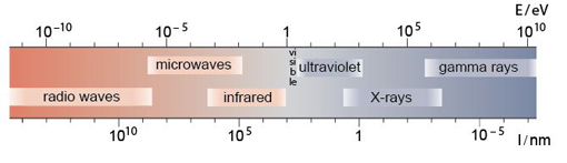
Light is a form of electromagnetic radiation, but it is only a small part (the visible part) of the whole electromagnetic spectrum, which also includes X-rays, ultraviolet and infrared radiation, and microwaves (Figure 26). The wavelengths of visible light span the region of the electromagnetic spectrum from about 400 nm (violet) to about 700 nm (red). Some of the properties of waves, with which you may already be familiar, are summarised in Box 2.
Box 2 Learn about light waves
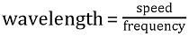
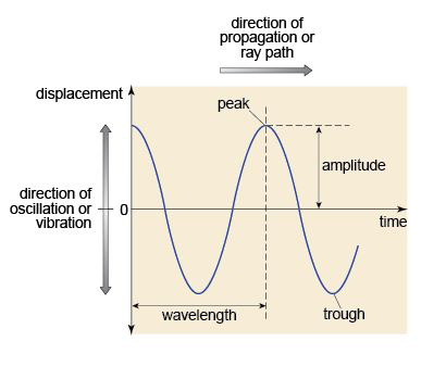
A wave is a disturbance that travels through a medium, transporting energy, but without permanent displacement of the medium. A wave moves by oscillations, which may be described as a regular sequence of peaks and troughs (like spreading ripples on a pond). The number of wave peaks that pass a fixed point per second is the frequency; and the distance between successive peaks is the wavelength (Figure 27). The wavelength depends on the frequency of the oscillation and the speed of propagation of the wave, according to the relationship:
The speed of a wave depends on the nature of the medium through which it travels - so, for example, the speed of sound in air is different from its speed in water.
2.1.1 Colour
Probably the most obvious property of a mineral is its colour. 'White' light contains a range of visible wavelengths from red to violet, but the mixture of colours is perceived to be white. When white light falls on an object some wavelengths are reflected, some are absorbed. The object then appears to be a particular colour because those absorbed wavelengths are missing from the reflected spectrum. The same happens when light passes through an object, which is the case with transparent and translucent minerals. A given crystal absorbs a particular range of wavelengths so that the colour of the light emerging from it depends on the type of mineral it is.
2.1.2 Refraction
When light passes from one transparent medium to another of different density, its speed changes. This effect is known as refraction. It is the reason that a straight stick emerging from water appears bent at the surface of the water, and why water viewed from above appears shallower than it really is. The change in the speed of light between air and the medium, expressed as a ratio, is the refractive index of the medium. (Note that this is a simplification. Strictly, refractive index is defined as the ratio of the speed of light in a vacuum to its speed in the medium. However, the speed of light in air is very close to that in a vacuum.)
2.2 Minerals and polarised light
A beam of light from an ordinary source, such as the Sun, consists of electromagnetic waves that vibrate in all directions at 90° to its direction of travel (Figure 28). Such a beam of unpolarised light can be modified to constrain its vibration direction to a single plane by using a polarising filter (a transparent sheet branded as Polaroid). Light transmitted through this polarising filter (or polariser) is called plane-polarised light (Figure 28). The direction of polarisation is the permitted vibration direction of the material. This effect is the basis for various observations using the polarising microscope that are important for identifying minerals.

2.2.1 Isotropic and anisotropic materials
Materials that have the same atomic structure in all directions are termed isotropic. When light passes through such a material it doesn't matter in which direction the light vibrates, its speed (and therefore the refractive index) is the same. This is true of light passing through air, water, glass and some minerals.
-
To which crystal system would you expect an isotropic mineral to belong?
-
The cubic system, because it defines materials for which the crystal structure and, consequently, its optical properties are the same along each crystallographic axis.
Minerals belonging to other crystal systems are more common than those with cubic symmetry. They have internal structures that are not the same along all crystallographic axes and are therefore anisotropic minerals. The importance of this is that the behaviour of the light passing through an anisotropic crystal depends on the vibration direction of the light and its relationship to the crystal structure.
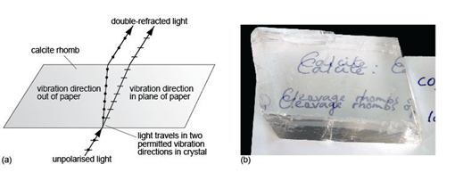
2.2.2 Double refraction
Anisotropic crystals have a remarkable property: when plane-polarised light enters such a crystal, it splits into two rays. The explanation for this involves complex crystal physics, which is well beyond the scope of this course. Nevertheless, the consequences are profound. The two rays are each plane-polarised, but their planes of polarisation (i.e. their vibration directions) are at 90° to each other. This means that each ray encounters a different atomic arrangement and therefore travels at a different speed through the crystal - so they have different refractive indices. The difference in refractive index of the two rays is called birefringence. If the refractive indices are very different (i.e. the crystal has a very high birefringence), then the two rays will be refracted to very different extents, and it may be possible to view two distinct images through the crystal, one for each ray. This effect, called double refraction, can be seen in the transparent variety of calcite, Iceland spar (Figure 29).
-
Would you expect to see double refraction in a cubic crystal?
-
No. Cubic crystals are isotropic. Double refraction occurs only in anisotropic crystals.
2.2.3 Pleochroism
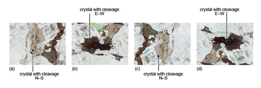
When plane-polarised light passes through an isotropic crystal, where the properties of the crystal are the same in all crystallographic directions, the colour of the transmitted light (due to the absorption characteristics of the crystal, Section 2.1.1) doesn't change as the crystal is rotated. However, when plane-polarised light passes through some, but not all, anisotropic crystals, and splits (Section 2.2.2), the light interacts with different arrangements of atoms with different absorption characteristics as the crystal is rotated, thus affecting the crystal's colour.
As an example, Figure 30a shows a very thin slice of biotite (a common rock-forming mineral) which has a faint beige colour when viewed in plane-polarised light and the cleavage is north-south. On rotating the mineral through 90°, the colour gradually changes to deep brown when the cleavage is east-west (Figure 30b). The same effects are repeated in Figures 30c and d. This property, whereby the colour of a mineral varies on rotation in plane-polarised light, is called pleochroism.
2.2.4 Extinction positions
When two polarising filters are held up to the light and their permitted vibration directions are parallel, light is transmitted. If one of the filters is then rotated through 360º, there will be two positions (at 90º and 270°) when the vibration directions are at right angles to one another, and at which no light is transmitted. In these positions, the polarisers (often called polars) are thus said to be crossed.
-
How would the intensity of any transmitted light change if an isotropic crystal was rotated between two crossed polars?
-
No light would be transmitted, irrespective of the orientation of the crystal. Thus isotropic minerals always appear black when viewed between crossed polars.
If an anisotropic mineral is placed between the crossed polars, the result is quite different. On entering the crystal, the plane-polarised beam splits into two plane-polarised beams at right angles to each other, constrained to the permitted vibration directions of the crystal. When a permitted vibration direction is parallel to the plane of polarisation of the beam, however, the beam does not split and the polarised beam is transmitted in that same plane. On emerging, this beam is effectively blocked by the other (crossed) polariser. As this happens for both permitted directions of the crystal, and as each is parallel to the plane of polarisation twice in a full 360° revolution, four extinction positions at 90° to each other are observable when an anisotropic mineral is rotated between crossed polars.
These effects are summarised in Figure 31. In (a)-(d), white light enters the first polarising filter and is polarised in the east-west plane. In each case this plane coincides with one of the permitted vibration directions in the mineral (when in the east-west position). Light then passes through the mineral, still polarised in the east-west plane. However, it is polarised at right angles to the permitted vibration direction of the second polariser, which therefore prevents the light from passing. Darkness results and the mineral is in extinction.
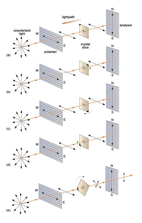
Figure 31e illustrates what happens between extinction positions. Light that has passed through the first polarising filter is polarised in the east-west plane as before. On entering the mineral it splits into two rays, polarised at right angles by the anisotropic mineral. These two rays then enter the second polariser. Their planes of polarisation are at an angle to the permitted direction of the second polariser, which constrains the transmitted component of each ray to the north-south plane, and so light passes through. The intensity of the transmitted light varies gradually from zero at the positions of extinction to a maximum at each position halfway between the extinction positions.
2.2.5 Interference colours
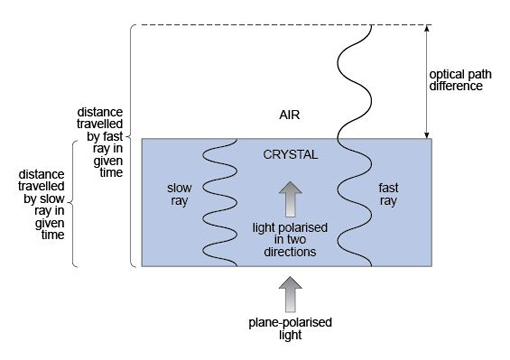
As you have seen, in between extinction positions light is transmitted through crossed polars (Figure 31e), but in an anisotropic mineral the two light rays would travel at different speeds in each permitted vibration direction. The second, crossed polariser effectively combines the two rays, but as they have travelled at different speeds through the mineral, they arrive out of step, to an extent (called the optical path difference) that depends on the difference in refraction (the birefringence) and the thickness of the mineral (Figure 32). Consequently, the transmitted light is no longer the mixture of colours that makes white light, but is a single interference colour as a result of interference effects between the two waves when recombined. The theory associated with production of interference colours need not concern you here, but the consequences are important.
The interference colour observed depends on the optical path difference and hence both the thickness of the mineral and the birefringence of the crystal in its particular orientation. A whole range of these interference colours can be seen when viewing a shallow wedge of quartz between crossed polars. Effectively, because the thickness of the wedge changes gradually while the birefringence remains the same throughout, the sequence of colours is a consequence of the transmitted rays becoming more and more out of step. The result is a 'spectrum' of interference colours called Newton's scale of colours - depicted on the Michel-Levy chart in Figure 33.

If the thickness of minerals to be observed were held constant, then the interference colours of the transmitted light would depend only on the difference in the refractive indices (the birefringence) for the light path in a given crystal. To see the more distinct interference colours shown in the left side of the chart (Figure 33), produced at the thin end of the wedge, the waves must not be too far out of step, so the mineral path must be short. In practice, slices of rock ground down to a thickness of just 30 µm ensure the transparency of most minerals, yet are sufficiently thick for distinct interference colours to be visible. By using this standard thickness of rock slices prepared for optical microscopy, uniformity is maintained, so that all observations of optical features are consistent from mineral to mineral and rock slice to rock slice.
The colour scale of the Michel-Levy chart can be divided into sections, called orders, separated by pinkish-purple bands (Figure 33). The more distinct colours at the thin end of the wedge are called low-order colours, and the lighter, less distinct colours at the thicker end are called high-order colours. For a slice of constant thickness, higher-order colours are produced by a mineral exhibiting higher birefringence. Calcite, with its high degree of anisotropy, is such a mineral.
When looking at interference colours, it is important to be aware of possible ambiguity in using the Michel-Levy chart. Some colours - particularly yellows and greens - appear in several places (i.e. in different orders) on the chart. Sometimes it can be difficult to establish the order of a particular interference colour. In general, higher-order colours appear much more washed out and pastel-like than lower-order colours, which are brighter and more vivid (Figure 33).
The refractive indices of an anisotropic mineral are related to its crystallographic axes and so its birefringence will vary according to its crystallographic orientation. This is an important point. If a single crystal of a mineral were taken and sliced in many different orientations, the interference colour would be different for each section - even for sections of the same thickness. In a rock that contains crystals of the same mineral in many different orientations, there will be differences in refractive index, hence birefringence, so that many different interference colours will be observed. However, the extent to which refractive indices can vary, and therefore the range of birefringence, is limited for any given mineral. In practice, it is the greatest difference in refractive index (i.e. the largest birefringence) and the maximum interference colour that can be identified, that is taken as characteristic (and can be diagnostic) of a particular mineral.
However, for some anisotropic minerals, slices can be cut in such a way that the refractive indices of the two plane-polarised rays are the same. This applies to minerals of the tetragonal, hexagonal and trigonal systems, when looking down their long (z) axes. Such a slice is often referred to as a basal section.
-
How would such a mineral, sliced perpendicular to its long axis, appear between crossed polars?
-
It would be in darkness throughout when rotated, just like an isotropic mineral.
-
What would be the range of interference colours visible for such a mineral present as grains in random orientations?
-
They would range from a maximum interference colour down through a range of intervening colours on the Michel-Levy chart to black.
2.3 Minerals and the polarising microscope
2.3.1 Introduction to the polarising microscope
The polarising microscope enables the examination of mineral grains and observation of the properties outlined in Section 2.2. A polarising microscope is very similar to an ordinary microscope except that it has two polarising filters and a rotating stage on which the sample is placed. Figure 34 illustrates a typical layout. Plane-polarised light is produced by passing white light through a polarising filter (the polariser) located beneath the rotating stage.
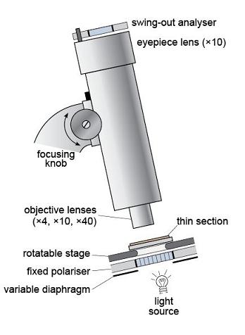
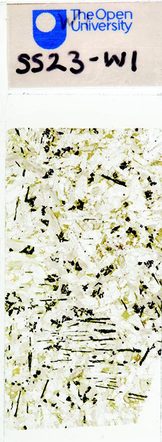
The plane-polarised light then passes through the sample, which is presented as a thin slice of rock, 30 µm thick, mounted on a glass slide - this is a thin section (Figure 35). A magnified image is produced using two sets of lenses: a lower, objective lens, and an upper, eyepiece lens. The magnification can be varied by changing the objective lens. The image is focused by moving the lens assembly up or down, using the focusing knob. It is usual to start by looking at a thin section using plane-polarised light and low magnification. After this, the second polarising filter, the analyser, can be inserted to view the specimen between crossed polars.
In this course, the Virtual Microscope substitutes for the polarising microscope. You will have the opportunity to familiarise yourself with the features and functionality of the Virtual Microscope in Activity 2.1.
The process of creating virtual microscope slides for Earth science creates image files of roughly 1GB for each thin section specimen using a motorised XY stage on a Leica DM4000M microscope. Rotation movies are digitised using an in-house system motorised Leica DM RP microscope.
Activity 2.1 Introduction to the Virtual Microscope
Task 1
This activity introduces you to the interface and functionality of the Virtual Microscope.
During this course, you will be using the Virtual Microscope, a system for viewing and exploring microscope slides (thin sections) of rocks using a computer and an internet browser window. The Virtual Microscope reproduces, and in some cases extends, the capabilities of the real microscope.
Open the Virtual Microscope and you should see a screen similar to the one shown in Figures 36 and 37. We will use the gabbro thin section to illustrate the Virtual Microscope, but this may not be the image that appears the first time you access the Virtual Microscope.
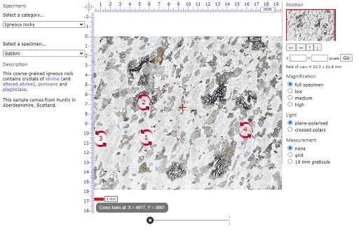
The screen is divided into a main viewing window and several functional areas that provide the ability to pan around the thin section, change magnification and light transmission conditions, and allow measurement (Figure 36).
In the upper left-hand corner, the catalogue of specimens can be accessed via two drop-down menus. The upper menu allows you to choose a sample category from the collection of geological thin sections, including different rock types, characteristic examples of particular minerals and various diagnostic features. The lower menu is a list of links to all the samples within your chosen category. You can use the collection to reinforce your learning and for reference during your Virtual Microscope studies.
Clicking and scrolling down the upper menu allows you to select from the menu of grouped igneous, metamorphic and sedimentary rocks, a cleavage slice of gypsum, rocks associated with a mapping activity later in the course, or a series of 'unknown' thin sections. There are also many other specimens that are not used in this course. Select 'Gabbro' in the 'Igneous' category for this demonstration.

Gabbro
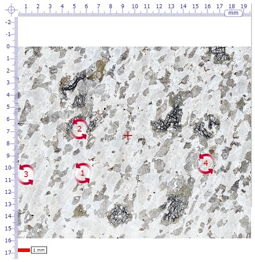
The main window shows the full thin section view when initially selected from the menu. In the middle of the field of view there is a small cross (traditionally called the 'cross hairs' because real hairs were used in early microscopes); this is used for locating features in the specimen (see point 5).
Note that a small number of red, numbered, circular arrows are visible. These are 'hot spot icons' that, when clicked, open a new window displaying rotatable images for viewing in plane-polarised light (left-hand circle), and between crossed polars (right-hand circle) (Figure 37).
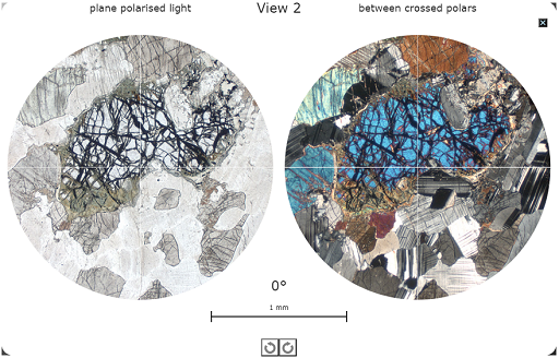 Figure 37 A view of one of the rotatable views (View 2) for the Gabbro page in the Virtual Microscope.
Click the small black box with a white cross in the top right-hand corner of this screen to return to the main viewing window
The image in the main window can be manipulated either by zooming in and out, or by panning around the specimen at selected magnifications. As the main image is zoomed or panned, the thumbnail image in the top right-hand corner shows the location of the main window as a red rectangle superimposed on the thumbnail image. The dimensions of the field of view of the main window are given in millimetres on the right above the image ‘Magnification’ heading.
The image can be moved in several different ways by:
- clicking and dragging the image itself
- using the four arrows on the right below the thumbnail image (further explained in point 6)
- clicking and dragging the red rectangle on the thumbnail image in the top right-hand corner
The image magnification can be changed in various ways:
- If you wish to zoom in on the current position of the cross-hairs, simply double-click anywhere within the field of view. Another double-click zooms in further.
- Zooming in and out can also be achieved using a mouse scroll wheel (if available), or the computer keyboard. Press the 'A' key to zoom in, and the 'Z' key to zoom out.
- A slider below the main viewing window can be used to zoom in and out; see point 6.
- Finally, there is a set of fixed magnifications, similar to a series of fixed objective lenses in a real polarising microscope, that can be used to standardise magnifications for some activities; see point 8.
A scale bar below the main view window on the left shows 1 millimetre.
From the main viewing window for gabbro, click on the red arrowed circle labelled ‘2’. The window that appears will display two circular images known as 'rotating views'. At this point, two high-resolution animations are loaded into the browser. The circles may be blank while this is happening.
- the view on the left is an area of the thin section displayed in plane-polarised light
- the view on the right is the same area of the thin section displayed as it appears between crossed polars.
The high-resolution animations may take several seconds to load, but take considerably longer over a slow internet link.
These rotating views are used to demonstrate several of the key optical properties of minerals in the thin sections: in plane-polarised light (PPL) and between crossed polars (XP). They can also be used to measure angles using the simple numerical indicator that lies centrally above the 1 mm scale bar.
The images in these views (i.e. PPL or XP) can be rotated to view changing colours (pleochroism or interference colours) and extinction by clicking and dragging either image using the mouse, or by clicking one of the circular arrows located below the 1 mm scale bar at the bottom of the screen.
Click the small black box with a white cross in the top right-hand corner of this screen to return to the main viewing window.
The location of the cross hairs is constantly displayed below the viewing window as X and Y coordinates. The sample can be moved to a specific location by typing the X and Y coordinates into the boxes and clicking the 'Go' button or by pressing the return key on the keyboard. This useful feature allows locations of particular features to be specified and communicated between different users.

Below and to the right-hand side of the main viewing window are a series of image manipulation controls. Use the slider at the bottom of the window to zoom in (right) and out:
Click on the arrows to the right of the window to move the viewing window across the thin section in the direction indicated.

We recommend that you try all the ways of moving the thin section and changing its magnification, to see which are best for you.
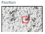
At the top right-hand side of the main window, a thumbnail image of the main window displays a red rectangle showing the location of the current field of view within the thin section as a whole.
Fixed magnifications are required for some tasks, and can also be used to switch quickly between magnifications and compare grain sizes at the same magnification in different thin sections.
Each thin section can be viewed in plane-polarised light and between crossed polars. Switch between the two views using the labelled buttons.

To the lower right of the thin section view are two tick boxes labelled 'grid' and '10 mm graticule'.

When the '10 mm graticule' box is selected, a 10 mm graticule with 0.1 mm divisions is superimposed over the thin section view, allowing direct measurement of features anywhere in the thin section once the features are moved to the centre of the field of view.
Two curved arrows rotate the graticule and grid to measure features in any orientation.
When the 'grid' box is selected, a grid that does not change in size with magnification is superimposed on the thin section view. The grid can be used to define an area for study at a particular magnification, and is especially useful to estimate proportions of different minerals in a view
The colour of the cross hairs and scale bar can be changed by clicking on the 'overlay colour' tick box.

To the left of the thin section view, a description of the rock and its locality are given for each thin section. Minerals and features that appear in blue are hyperlinks to examples in the thin section, many of which are shown in the rotating views.
Click 'olivine' in the gabbro description and the thin section view changes to display olivine at an appropriate magnification.
Questions 2.1.1 and 2.1.2 use the Virtual Microscope to view a virtual gypsum cleavage slice ('Miscellaneous' category). You may wish to reflect on the similarities between the two ways of seeing the same phenomenon and additional things you can observe using the Virtual Microscope.
Question 2.1.1
Select the 'Gypsum cleavage slice' from the ‘Miscellaneous’ category of the Virtual Microscope. The single rhomb-shaped crystal fills most of the field of view even at low magnification. By default, the first view will be in plain polarised light. Now select the view between crossed polars. Ignoring the crystal for the moment, why is the field of view outside the boundaries of the crystal clear or transparent in plain polarised light but black when viewed between crossed polars?
Answer
This view corresponds to observation of the gypsum slice between the two sheets of polarised material. (Remember that you learned about minerals and polarised light in Section 2.2.) In plain polarised light, the glass slide on which the gypsum slice is mounted is transparent; however, when viewed between two pieces of polarised material with their polarising directions at right angles, the background and the glass slide appear black. This is because the light is polarised in one direction by the first sheet of polarising material and that direction is blocked by the second, thus allowing no light to pass.
Question 2.1.2
Now consider the crystal slice in the view between crossed polars for the single crystal of gypsum. Given that this is part of a single crystal of gypsum, can you explain the reason for the range of interference colours you observe?
Answer
This cleavage fragment exhibits a wide range of interference colours (including low-order colours at the grain margins on the left-hand side) that correspond with the colours in the Michelle Levy chart of interference colours in Section 2.2.5. This is because it is not a true thin section with a uniform 30 μm thickness, but a broken fragment of a crystal with variable thickness presenting different path lengths to light passing through different parts of it. At its thinnest points close to the edge, the crystal exhibits first-order interference colours, whereas the thicker areas in the centre of the crystal exhibit third and fourth order colours.
Question 2.1.3
Returning to the plane-polarised view, in the main window, click the red-arrowed circle (numbered 1) to open the rotating views in a new window. Explain what you observe as you rotate this part of the gypsum slice in (a) plane-polarised light and (b) between crossed polars.
Answer
- a.On rotation in plane-polarised light, the appearance of the gypsum crystal slice remains the same except for changing from slightly darker to lighter due to varying relief, rather than pleochroism; the darkness of the glass mount beyond the crystal slice also changes very slightly too.
- b.On rotation between crossed polars, the interference colours remain the same, although the brightness varies: every 90°, the crystal slice becomes completely dark. Thus, the crystal slice goes dark four times per complete rotation. The glass slide visible beyond the edge of the crystal slice remains dark in all orientations, as glass is isotropic. When the gypsum cleavage slice is in extinction, you may observe dust on the section and at least one small fragment of gypsum in a different orientation that still shows low-order interference colours when the main crystal is in extinction. In fact, you may also notice that this fragment never goes into extinction because two crystals on top of each other are very unlikely to be completely aligned with the polarisers. One of the reasons that geologists use very thin slices of rock is to avoid this effect and to observe the optical properties of individual crystals in thin section.
2.3.2 Minerals in thin section
Microscopic examination of a rock in thin section enables its constituent minerals and its textural properties to be identified. These are important and essential steps in establishing a rock's identity and in deducing how it was formed. The Virtual Microscope is designed to provide images as would be seen using a real polarising microscope. Views of numerous rock thin sections are available in plane-polarised light (PPL) and between crossed polars (XP), at different magnifications and at selected rotation points. The main optical properties used to identify minerals in both plane-polarised light and between crossed polars are outlined below. You can view examples of all these properties in the ‘Mineralogical features’ category of the Virtual Microscope.
In plane-polarised light
Relief. Relief is the term used to describe the degree to which edges and surface imperfections of crystals are visible in plane-polarised light. Minerals with a refractive index very different from that of the mounting glue are said to have high relief as they appear to 'stand out' from the slide (as for pyroxene in Figure 38a): grain boundaries are easily seen and surface imperfections appear pronounced. Minerals with refractive indices similar to that of the mounting glue are said to have low relief: individual grain boundaries are not easily observed and the minerals are featureless and almost invisible in plane-polarised light (as for plagioclase in Figure 38b). If the mineral is highly anisotropic (e.g. calcite), the relief may vary as the stage is rotated: the transmitted light sampling first one permitted vibration direction, then the other.
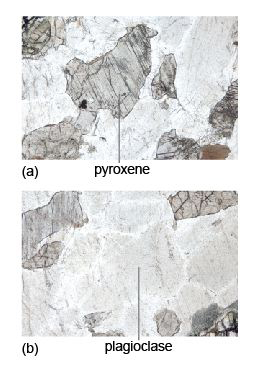
Cleavage. Cleavage traces may be seen as sets of parallel straight lines cutting through a mineral section (Figure 38a). The presence, number and angular relationships of cleavage traces can be diagnostic for some minerals. Micas have one good strong cleavage (Figure 10c); pyroxenes and amphiboles have two cleavage planes, which intersect at about 90º and 120º, respectively, when basal sections are viewed in cross-section (Figure 42).
Colour and pleochroism. Many coloured silicate minerals are rich in iron (e.g. ferromagnesian minerals). If the colour changes as the mineral is rotated in plane-polarised light, the mineral is said to be pleochroic (i.e. the mineral absorbs light differently in different orientations - a concept met in Section 2.2.3). Biotite (dark mica) and amphiboles are good examples of pleochroic minerals, biotite commonly having characteristic pale- to dark-brown pleochroism (Figure 30).
Opaque minerals. Many opaque minerals are metal oxides, such as hematite (Fe2O3) and ilmenite (FeTiO3), or sulfides, such as pyrite (FeS2). Opaque minerals transmit no light - even in 30 µm thin sections: they appear black when viewed in both plane-polarised light and between crossed polars (in any orientation). Opaque minerals should not be confused with non-opaque minerals that are isotropic and appear black only between crossed polars.
Between crossed polars
Isotropic minerals. Isotropic minerals (e.g. garnet and fluorite) belong to the cubic system and, like glass, which is a disordered solid (Section 2.2), always appear black between crossed polars (e.g. the garnet in Figure 44c), regardless of their orientation but, unlike opaque minerals, will transmit light when viewed in plane-polarised light.
Anisotropic minerals. An anisotropic mineral (most minerals) will normally display an interference colour when viewed between crossed polars and will pass in and out of extinction (at 90° intervals) as the stage is rotated. The interference colour depends on the crystallographic orientation of the mineral. When an anisotropic mineral is viewed in an orientation whereby the refractive indices in the permitted directions are the same (i.e. down the long axes of tetragonal, hexagonal and trigonal minerals), the mineral appears dark as the stage is rotated (i.e. it behaves like an isotropic mineral). This would be a basal section.
Interference colour. The Michel-Levy chart is used to estimate whether a mineral has high-order or low-order interference colours. When several grains of the same mineral are present, it is necessary to look for the one that shows the highest-order interference colour, which corresponds to the maximum birefringence.
Extinction. Cleavage traces can also be observed between crossed polars. Because cleavage planes are usually related to crystallographic axes, there is often a relationship between cleavage direction and the position at which the mineral goes into extinction. When cleavage traces are parallel or perpendicular to a mineral's permitted vibration directions, the extinction position is parallel to the cleavage and is referred to as straight extinction. When the extinction position is at an angle to the cleavage trace, the mineral shows inclined extinction.
Twinning. A twinned crystal consists of regions that are structurally related to each other across a twin plane (Section 1.5). These regions are called twin components and, when viewed between crossed polars, adjacent components will go into extinction in different positions. Simple twins comprise just two components, side by side. However, some minerals (e.g. plagioclase feldspar), feature multiple twin components and, when viewed between crossed polars, have a striped appearance (Figure 19c). Rotating the crystal causes the bright and dark stripes to swap over.
Activity 2.2 Exploring mineral properties in thin section
Task 1
For this activity you will require the Virtual Microscope. Use the drop-down menus of categories and sample names to navigate to the thin sections specified.
Question 2.2.1
Look at the thin section of quartzite in plane-polarised light (which can be found under the ‘Metamorphic rocks’ category). It contains many different grains of the same mineral (quartz). Can you see any boundaries between grains? Why are they not very clear? Now select crossed polars. Can you distinguish between different grains more easily? If so, what is the explanation for this?
Answer
Grain boundaries are quite difficult to see in this thin section because it contains just one kind of mineral, quartz, which has very low relief. The grain boundaries are much more evident between crossed polars: different quartz crystals are in different orientations, hence have different birefringence and show different interference colours.
Question 2.2.2
Examine the thin section of peridotite (which can be found under the ‘Igneous rocks’ category), first in plane-polarised light, then between crossed polars. It contains abundant grains of the mineral olivine. How do (a) relief and (b) interference colours of olivine compare with those seen in the quartzite?
Answer
Compared with the quartz crystals in the quartzite, the olivine crystals in the peridotite show (a) higher relief in plane-polarised light and (b) higher-order interference colours between crossed polars.
Question 2.2.3
Look at the granite thin section (which can be found under the ‘Igneous rocks’ category) in plane-polarised light. Note the brown mineral. Select one of the rotating view hot spots containing the mineral. What happens to the colour of this mineral when it is rotated in plane-polarised light? What is this phenomenon called? What is its origin?
Answer
In plane-polarised light, the colour of the brown mineral (biotite) changes as the slide is rotated. This phenomenon is called pleochroism; it is caused by a variation in the absorption of light, depending on the orientation of the crystal relative to the polarisation direction.
Question 2.2.4
Look at the thin section of schist (which can be found under the ‘Metamorphic rocks’ category). Note the large, equidimensional (garnet) crystals in plane-polarised light. These crystals seem to stand out from the slide and have more surface texture than the surrounding minerals. They are said to have high relief. How does the relief of these crystals compare with the relief of the other crystals in the slide? Now look at the thin section between crossed polars. What happens to the garnet crystals when the stage is rotated? What term describes crystals that exhibit this property? From this optical behaviour, what is the crystal system of garnet?
Answer
The garnet crystals have much higher relief than the other crystals. Viewed between crossed polars, the garnet crystals are black, and remain so as the stage is rotated, whilst the other crystals display a variety of interference colours ranging from low-order to high-order colours. The garnet crystals are therefore optically isotropic, and so must belong to the cubic system.
The next section will focus on the recognition of the main rock-forming minerals using these properties. You can find many more rocks presented on the Virtual Microscope collections website, created by The Open University in partnership with several other organisations with funding from JISC.
Although optical microscopy still has great value, providing an essential contextual framework for studying minerals and deducing how their characteristics and interrelationships reveal the manner of their formation, there are today many sophisticated procedures that can be used to extend our knowledge of minerals. A flavour of some of these is provided in Box 3.
Box 3 Determining mineral chemistry
Nowadays, interpreting the behaviour of rocks during their formation and subsequent events requires the chemical composition of their constituent minerals to be quantified. This can be done with modern instrumentation. In particular it can be important to determine the composition of individual grains, and even the variation within a grain. Appropriate modern microanalytical techniques use the electron microprobe (EMP), laser ablation inductively coupled plasma mass spectrometry (LA-ICP-MS) and the ion microprobe (IMP).
The electron microprobe technique involves directing a focused electron beam at a polished surface of a mineral grain. X-rays that are specific for each constituent element are emitted from the mineral. By measuring the intensity of the X-rays that characterise different elements, the major and minor element composition of 'spots' only a few μm across can be obtained. Alternatively, the beam may be scanned across the surface of mineral grains to produce X-ray maps of elemental concentrations. Another way of mapping minerals is by back-scattered electron (BSE) imaging. This is an image of the electrons that are scattered or bounced back by atoms bombarded by the electron beam. The number of electrons back-scattered is proportional to the mean atomic mass of the spot under the beam. So, brighter areas of the image represent minerals containing heavier elements (e.g. Fe and Ca) and darker areas represent minerals containing lighter elements (e.g. Si, Al, Mg and Na) (see Figure 39).
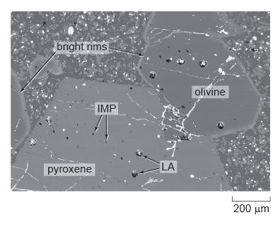
LA-ICP-MS uses a laser probe to melt a hole in a mineral; the vaporised (ablated) material is then analysed by mass spectrometer for its trace element, and sometimes its isotope, compositions. Spot sizes are 40-100 μm; which is generally larger than those of the EMP, but lower concentrations can be determined.
The ion microprobe uses an ion beam to remove (sputter) very small amounts of material from a spot 100 nm to 40 μm in size. The sputtered material is then analysed by mass spectrometer for its isotope and trace element compositions.
These micro-analytical techniques can be used to investigate the crystallisation history of an igneous rock. The back-scattered electron image in Figure 39 shows several large crystals of the minerals olivine and pyroxene surrounded by finer-grained crystals in a lava from the Solomon Islands in the western Pacific. EMP analysis reveals (Figure 40) that the bright rim around the edge of the olivine crystals is rich in iron, but the iron content decreases inwards until, from about 50 μm in from the rim, through the central part of the grain, the olivine has a constant (magnesium-rich) composition. This chemical profile is interpreted as being due to the diffusion of iron and magnesium between the surrounding magma and the olivine crystal just prior to eruption of the lava. The large pyroxene crystal also has a regular compositional variation around its edges, but this can be revealed only by LA-ICP-MS and IMP analysis of the trace element contents, which increase near the edge of the crystal.
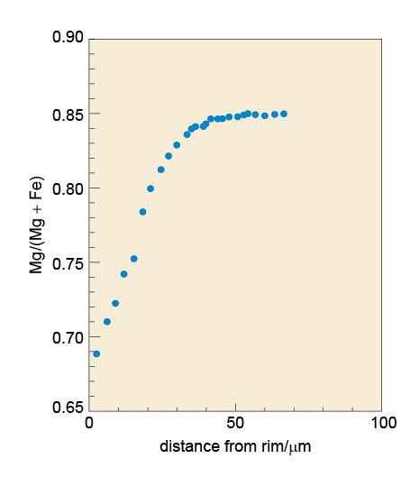
If the temperature of the lava is known (by calculation from the chemistry of the lava and the minerals), it is possible to use the diffusion profile (the compositional gradient) in the rim to calculate how long the crystals had resided in the melt just prior to eruption. In this example, diffusion modelling reveals that the large crystals were there for 13.8 ± 1.4 days at a temperature of 1100 °C. This was long enough to produce the iron-rich rim of the olivine. The uniform internal compositions indicate that these crystals had originally crystallised elsewhere in the magmatic system.
2.4 Summary of Section 2
- Light consists of electromagnetic waves that vibrate in all directions at 90° to the direction of travel of the light beam. White light is a mixture of coloured light with a range of frequencies.
- The change in speed of light as it travels between media of different densities is known as refraction. The ratio of the speed of light in a given medium and its speed in air (strictly, in a vacuum) is the refractive index of that medium.
- A polarising filter allows light to pass through, vibrating in one plane known as the permitted vibration direction. The light is plane-polarised.
- Plane-polarised light passing through an anisotropic mineral splits into two plane-polarised rays that vibrate at 90º to each other. These rays travel at different speeds and give rise to double refraction, a property that is well developed in transparent calcite rhombs.
- In plane-polarised light, some minerals absorb different wavelengths of light depending on the orientation of the crystal. This produces colours that vary with crystal orientation: a property known as pleochroism.
- When an isotropic crystal (with the same optical properties in all directions) is placed between two polarising filters with their permitted vibration directions at 90° (i.e. crossed polars), no light will pass through, irrespective of the mineral's orientation (it appears uniformly black on rotation). Cubic minerals show this effect.
- When an anisotropic crystal (with different optical properties in different crystallographic directions) is placed between two polarising filters and the mineral is rotated through 360º, there are four positions of darkness (extinction positions) that are 90º apart, between which the mineral appears coloured (has an interference colour) with an intensity that peaks halfway between extinction positions.
- The difference in refractive index of light rays passing along the permitted vibration directions of an anisotropic mineral is its birefringence. When two such rays emerge, they are out of step, and when recombined on passing through a second, crossed polariser, interference colours are produced.
- The sequence of interference colours as produced by increasing birefringence and simulated by a quartz wedge is represented on a Michel-Levy chart. Maximum interference colours can be diagnostic of particular minerals.
- Opaque minerals do not transmit light of any kind.
- A polarising microscope with a rotating stage and two polarising filters provides the facility to observe a range of diagnostic optical properties for mineral grains presented as a thin slice, 30 µm thick. Such rock slices mounted on glass are known as thin sections.
- Other key diagnostic optical properties of minerals include relief, cleavage traces and twinning.
2.5 Learning outcomes for Section 2
Now you have completed this section, you should be able to:
- suggest different ways in which light passing through a crystalline material is modified
- define the terms refractive index and birefringence
- explain the meaning of the terms isotropic and anisotropic, permitted vibration direction, double refraction and pleochroism
- describe how plane-polarised light passes through an anisotropic crystal on the stage of a polarising microscope
- explain the origin of interference colours in anisotropic materials
- describe how to identify an unknown mineral (in thin section) using a polarising microscope.
Now try the following questions to test your understanding of Section 2.
SAQ 4
A slice of an unknown mineral has been examined with a polarising microscope. In plane-polarised light the mineral appeared colourless, but when viewed between crossed polars it appeared dark, and remained dark as the mineral was rotated. To what crystal system is this mineral likely to belong?
SAQ 5
In plane-polarised light, a thin section of a mineral shows very high relief, but as the stage is rotated through 90°, this changes to very low relief. Why does the relief change with orientation? What prediction can you make about the interference colour for this mineral?
SAQ 6
In Section 1, you were introduced to the crystal structures of two polymorphs of carbon: diamond and graphite. Based on your knowledge of these structures, what prediction(s) can you make about the optical properties of diamond and graphite?
3 Rock-forming minerals
3.1 Introduction
More than 90 chemical elements occur naturally on Earth. You might expect them to combine in ways that would form an almost infinite number of minerals. In fact, the total number of minerals discovered is only about 4000, and the number of commonly occurring rock-forming minerals is very much smaller. One reason for so few common minerals is that most elements have low abundances and rarely occur in sufficient quantities to combine and form minerals. Thus the more widely occurring rock-forming minerals represent combinations of a small number of readily available ingredients, those elements which are more abundant in the Earth's crust and mantle, as listed in Table 4.
| Element | Symbol | % in crust (by mass) | % in mantle (by mass) |
|---|---|---|---|
| oxygen | O | 46.6 | 44.6 |
| silicon | Si | 27.7 | 21.4 |
| aluminium | Al | 8.3 | 2.2 |
| iron | Fe | 5.0 | 5.9 |
| calcium | Ca | 3.6 | 2.3 |
| sodium | Na | 2.8 | 0.2 |
| potassium | K | 2.6 | trace |
| magnesium | Mg | 2.1 | 22.7 |
| others | 1.3 | 0.7 | |
| total | 100.0 | 100.0 |
From Table 4, it is clear that oxygen and silicon are by far the most abundant elements in the crust and mantle. Minerals containing silicon combined with oxygen are called silicate minerals, and are the single most important mineral group - making up over 90% of the Earth's crust and almost all of the mantle.
The non-silicate minerals (of which calcite is perhaps the most familiar example) contain other chemical groups, such as carbon combined with oxygen (carbonates) and metals combined with oxygen (oxides) or sulfur (sulfides).
The following sections contain descriptions of the crystal structures of important rock-forming minerals. Note: you would not normally be expected to remember specific details of the structures, merely the essential attributes of, and differences between, the structures of the main mineral groups.
3.2 Silicate mineral structures
Silicate minerals all share the same basic building block: a silicon atom bonded to four oxygen atoms at the corners of a tetrahedron, called the silicate group (or SiO4 group) (Figure 41).
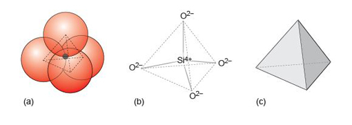
The wide range of silicate minerals that exists in nature owes much to a property of the SiO4 group, known as polymerisation. Polymerisation generally leads to increasingly complex mineral structures. At the simplest level, SiO4 groups bond with metal cations, forming isolated groups (Figure 42) as in olivine minerals (Section 3.3.1). With increasing polymerisation, the SiO4 group can also build two- and three-dimensional structures, such as chains, sheets and frameworks, by linking up SiO4 tetrahedra. With the exception of the silica minerals, where all the oxygens are shared, these structures are also linked by a variety of cations to make more complex three-dimensional structures.
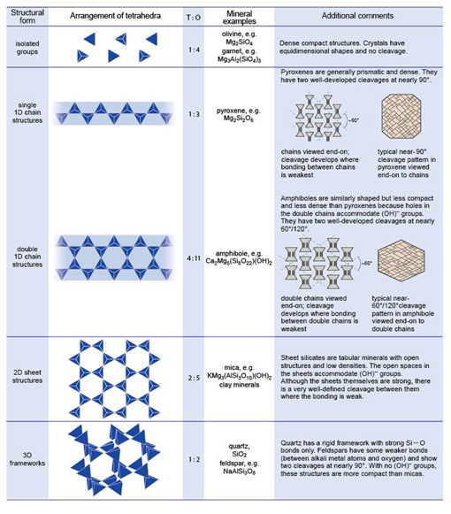
The first stage of polymerisation of SiO4 groups involves the formation of chain structures, as in pyroxene minerals (Section 3.4.1), produced by corner-sharing of the oxygen atoms (Figure 42). The ratio of silicon to oxygen atoms increases from 1 : 4 in structures with isolated SiO4 groups, to 1 : 3 in chain structures. The degree of polymerisation increases further in more complex chains (Figure 42), as in amphibole minerals (Section 3.4.2), and the ratio of silicon to oxygen increases to 4 : 11. Further polymerisation produces sheet structures, whereby tetrahedra are linked in two dimensions to form sheets (Figure 42). These sheets are bonded together by a variety of chemical groups, such as hydroxyl (OH−) or metal cations, to form sandwich structures and the Si : O ratio rises to 2 : 5. In fully polymerised three-dimensional framework structures, as in quartz (Section 3.6.1), the Si : O ratio reaches 1 : 2.
In some minerals, aluminium replaces silicon in some of the SiO4 tetrahedra producing AlO4 groups. It is therefore more appropriate to think of oxygen atoms being shared between tetrahedral (T) sites, which may contain either silicon or aluminium. So, more generally, increasing polymerisation results in an increase in the ratio of tetrahedral sites to oxygen - the T : O ratio (Figure 42). The net charge on the SiO4 group is −4, but on the AlO4 group it is −5, so additional positive charges are required to compensate for the excess negative charge on the tetrahedral groups. These may be provided by cations, commonly metals, residing in cavities or interstices in the tetrahedral structure (Section 1.4.2). Figure 42 summarises the structural styles of the major silicate mineral groups. In the following sections, you will look at each of these groups in more detail.
3.3 Minerals with isolated SiO4 tetrahedra
Minerals with isolated SiO4 tetrahedra have the simplest structures. They also have the lowest T : O ratio (i.e. 1 : 4).
3.3.1 Olivine
The name 'olivine' refers to a group of minerals with a continuous spread of chemical compositions between forsterite (Mg2SiO4) and fayalite (Fe2SiO4), and the formula is written as (Mg,Fe)2SiO4, indicating that atoms (in fact, ions) of magnesium and iron can substitute for each other. This kind of chemical mixture is called a solid solution and involves ions having similar sizes and similar charges (e.g. Mg2+ and Fe2+). For a complete solid solution, as developed between forsterite and fayalite, the substituting ions must have similar ionic radii (a measure of their size), so that either ion can fit into the same interstitial site in the crystal structure.
Olivine is an important example of a structure with isolated tetrahedra. Every SiO4 group has a net charge of −4 (Figure 41b), and because the crystal has to be electrically neutral, olivine contains two doubly charged (2+) cations per SiO4 unit. Silicon atoms reside in tetrahedral interstices (i.e. at the centres of SiO4 tetrahedra), whereas octahedral interstices contain the larger magnesium and iron atoms (Section 1.4.2). These are close-packed, largely ionic structures, which explains why, compared with other silicates, olivine has a relatively high density. The structure is also strong in three dimensions, making olivine a hard mineral, without any good cleavage. Olivine has a characteristic olive-green colour (Figure 43a) that becomes darker with increasing iron content.
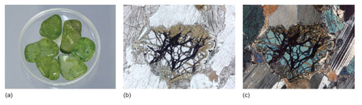
Olivine is stable at high temperatures and pressures, and forms about 60% of the Earth's upper mantle. It crystallises at high temperatures from magmas rich in iron and magnesium and relatively poor in silica (SiO2). In such rocks, where olivine is one of the first minerals to crystallise as the magma cools, it may develop well-formed crystals, surrounded by later-crystallising minerals (which tend to be smaller, and lack such ideal crystal shapes).
Olivine is prone to alteration at lower temperatures under hydrous conditions, especially during weathering. Under the microscope, evidence of this alteration in olivine crystals takes the form of new minerals, such as greenish or brownish serpentine, and curved, irregular cracks filled with iron oxide (opaque) (Figure 43b and c).
Activity 3.1 Olivine in hand specimen and thin section
Task 1
This activity will help you to recognise olivine in hand specimen and in thin section. For this activity you will require the Digital Kit and the Virtual Microscope.
- Examine the peridotite sample in the Digital Kit. If you could feel it, you'd notice that it feels much denser ('heavier') than other rocks of a similar size. The peridotite sample in the Digital Kit contains olivine that appears brownish-grey and translucent under lights (for photography) and the pyroxene is creamy bronze. The pyroxene can be recognised by its cleavage; but cleavage is lacking in olivine.
- Now use the Digital Kit to examine the gabbro. This rock contains pyroxene and plagioclase as well as olivine.
Question 3.1.1
Describe the textures you see in the gabbro and briefly try to explain the characteristic features that help to identify the minerals.
Answer
The mineral plagioclase is easiest to identify in the gabbro, since it has a white colour and tablular shape. Distinguishing between olivine and pyroxene is much more difficult. You may be able to identify cleavage in the pyroxene and the slightly paler brown colour compared with a more intense green of the olivine, but neither of these colours is entirely diagnostic. This is why geologists use the petrological microscope, where the two minerals have very different appearance to one another and are more easily distinguished.
Task 2
- Examine the gabbro thin section using the Virtual Microscope (under the ‘Igneous rocks’ category). You should become accustomed to using the views in plane-polarised light (PPL), between crossed polars (XP) and the rotations, which are often positioned on good examples of particular minerals. In PPL, the mineral with very high relief, but clear, and criss-crossed by often curved cracks, is olivine (View 2). The cracks here are enlarged and contain alteration products, mainly iron oxides, which exaggerate the appearance of the relief. The olivine is clearly distinguishable from pyroxene, which has more moderate relief and often shows a cleavage (View 1), whereas olivine has no cleavage. There are also green to brown, low-relief areas of alteration at the margins of some olivine crystals that are most probably the mineral serpentine (View 4).
- Now examine the peridotite thin section using the Virtual Microscope. The abundant olivine crystals are more difficult to distinguish from those of pyroxene than they are in the gabbro, because their relief is similar. The olivine can usually be identified by the presence of curved cracks, lack of cleavage and, in XP view, they often have bright interference colours - up to second-order blue (e.g. at coordinates 3200,2230). The pyroxenes have a cleavage and their interference colours are mainly first-order (e.g. at coordinates 3900,2250).
3.3.2 Garnet
Like olivine, the garnet group of minerals is also based on a structure of isolated SiO4 tetrahedra and, as a result, garnets are also dense minerals and are commonly formed at high pressures both in the Earth's crust and mantle. Garnets are found in many crustal metamorphic rocks, especially those formed at depths greater than ~24 km, and are ubiquitous in the upper mantle at depths greater than 85 km. Garnets may also occur in some igneous rocks.
Although the garnet crystal structure is complex, it belongs to the cubic system, so garnets are optically isotropic (Figure 44c). Garnets have the general chemical formula A3B2(SiO4)3 where A represents divalent (2+) metal ions and B represents trivalent (3+) metal ions. However, garnets have a wide range of chemical compositions; they may contain various combinations from aluminium, calcium, iron, magnesium or even rare-earth elements, such as yttrium.
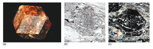
Activity 3.2 Garnet in hand specimen and thin section
Task 1
This activity will help you to recognise garnet in hand specimen and thin section. For this activity you will require the Digital Kit and the Virtual Microscope.
- Examine the schist using the Digital Kit. This rock contains several other minerals, apart from garnet, but you can identify the garnets as small, pinkish-red to deep wine-red crystals. Unlike the other minerals such as mica and quartz, however, the garnets have equidimensional shapes reflecting their crystal symmetry. Note that garnets can be different colours, which vary widely from green to red to brown and very dark reddish-brown.
Question 3.2.1
Garnet belongs to the cubic system. What prediction can you make about its optical properties?
Answer
Cubic crystals are optically isotropic. You can therefore predict that, when viewed between crossed polars, the garnet crystals will appear dark, and will remain dark as the crystal is rotated.
Task 2
- Examine the schist in thin section with the Virtual Microscope (which can be found under the ‘Metamorphic rocks’ category). Starting with plane-polarised light, note the high-relief garnet crystals, up to 4 mm across, which have almost equidimensional shapes. Note also the way that the surrounding minerals appear to 'flow' around the garnets. Now select crossed polars and verify that garnet crystals are isotropic (see Question 3.2.1). For further confirmation, select the View 1 rotation.
3.4 Chain silicates
3.4.1 Pyroxene
The pyroxene group of minerals has the general formula ABSi2O6 (where A and B refer to divalent metal ions in the A and B sites, respectively). Some pyroxenes belong to the monoclinic system; others to the orthorhombic system. Important clinopyroxenes (monoclinic) include augite (Ca(Mg,Fe)Si2O6), and orthopyroxenes (orthorhombic) include enstatite (Mg2Si2O6).
-
Which metal atoms occupy which sites in augite?
-
Using the general formula ABSi2O6, Ca occupies the A site, and the B site contains a mixture of Mg and Fe atoms. Note that the formula of augite implies that there is solid solution from CaMgSi2O6 to CaFeSi2O6.
All pyroxenes are formed of single chains of SiO4 tetrahedra, similar to that depicted in Figure 42. In three dimensions, the chains are interconnected via strong bonds to cations at the B site. The chains that are bonded by the B-site cations are then stacked together to form a strong structure. Adjacent chains mesh into each other and are weakly bonded by a second set of cations, residing in A sites, so for every two SiO3 chain units, there is one A site and one B site.
The differences between the A and B sites are important and are key to understanding the mechanical properties of pyroxene. The pyroxene structure is not uniformly strong and the regions between the chains are relatively weak such that they are likely to break - or cleave - along these directions. This gives two good cleavage directions at approximately 90° (strictly 87° (or 93°)) to each other (Figure 42).
-
When you observe pyroxene cleavages in thin section, will the traces always be at about 90° to each other?
-
The two sets of cleavage traces will only be at about 90° to each other if you are looking down the length of the crystal. This is the basal section for pyroxene. If you were looking perpendicular to this direction (i.e. sideways onto the length of the crystal), there would appear to be only one set of parallel cleavage traces. This is true of the crystal illustrated in Figure 45b. Note, however, that if you were looking obliquely to the basal section the cleavage traces would form a diamond-shaped outline.
In pyroxenes where one set of cleavage traces is visible in thin section (Figure 45b), it is easy to distinguish orthopyroxenes, with straight extinction, from clinopyroxenes, with inclined extinction.
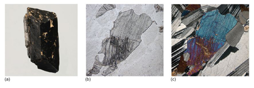
Pyroxenes are important rock-forming minerals commonly found in many igneous and metamorphic rocks. Pyroxenes in basaltic igneous rocks have different compositions from those in andesites. Their occurrence is more restricted in metamorphic rocks but they can be important in those formed at high temperatures.
3.4.2 Amphibole
The amphibole group of minerals is chemically more complex than the pyroxenes. The general formula can be written as AB2C5Si8O22(OH)2, where A represents a large cation such as Na, and B and C represent smaller cations, such as Ca or Mg. Amphiboles also contain the hydroxyl group, (OH), and are therefore hydrous minerals, in contrast to pyroxenes, which are anhydrous minerals.
Amphibole minerals contain double silicate chains (Figure 42) resembling the pyroxene structure, and likewise have two distinct cleavages. However, because these chains are wider than the pyroxene single chains, the cleavages intersect at about 60° or 120° (strictly 56° (or 124°)), as illustrated in Figures 42 and 46b.
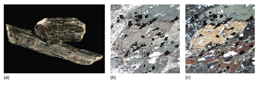
One way to distinguish amphibole from pyroxene in thin section is by its roughly 60° (or 120°) cleavage in basal sections (Figure 46). Most often the cleavage is parallel and amphiboles have inclined extinction. Some common varieties are strongly pleochroic (some with yellowish-green turning to brown colours; some are deep blue turning to colourless).
Amphiboles are found in many metamorphic rocks and crystallise from hydrous magmas (containing water) that have moderate to high SiO2 and Na2O contents, such as andesites.
Activity 3.3 Pyroxene and amphibole in hand specimen and thin section
Task 1
This activity focuses on the features by which pyroxene and amphibole can be distinguished in hand specimen and thin section. For this activity you will require the samples of gabbro and amphibolite in the Digital Kit and the Virtual Microscope.
- Pyroxene is a mafic mineral, and often forms green to black crystals (see Digital Kit examples). Gabbro contains olivine crystals (greenish-grey), feldspar (grey to white), and pyroxene (black). See if you can identify any pyroxene crystals in the gabbro or peridotite (the labels available in the Digital Kit can help you identify pyroxene) - they are visible in the close-up view in the Digital Kit.
Question 3.3.1
Considering the structure of pyroxene, would you expect this mineral to be optically isotropic or anisotropic?
Answer
Pyroxene has a chain structure, with the chains aligned in the same direction. Its optical properties are therefore different in different directions and the transmission of light is dependent on the direction of vibration. Consequently, you would expect it to be anisotropic.
Task 2
- Examine the thin section of gabbro using the Virtual Microscope (found under the ‘Igneous rocks’ category).. This rock contains a very low-relief mineral (seen in plane-polarised light), which is typically striped (due to twinning) when viewed between crossed polars. As you saw in Activity 3.1, it also contains olivine, which is distinctive with its very high relief (and characterised by its curved cracks), and pyroxene, with moderately high relief. Many of the pyroxene crystals show cleavage traces, and are only faintly coloured.
- Amphibole is another mafic mineral and typically forms dark-green to black prismatic crystals. An amphibolite, contains abundant amphibole.
Question 3.3.2
How is cleavage used to distinguish pyroxenes from amphiboles?
Answer
The pyroxene structure has weak bonding between the chains, giving rise to two sets of cleavage planes at about 90° (actually 87° (or 93°)) to each other (Figure 47a). In thin section, most often you can see only a single set of cleavage traces, e.g. View 1 rotation. In a basal section, if visible, two sets of traces (coloured blue and red in Figure 47a) can be seen at about 90° to each other. Basal cleavages at about 90° can be seen at one end of a pyroxene prism in the Digital Kit. Viewed from the side, both sets of cleavage planes are parallel to the length of the prism.Amphibole, like pyroxene, has a chain structure, with weak bonding between the chains. The chains are wider than in pyroxene (they are double chains), and the cleavage angle in basal section of an amphibole is about 60° (actually 56°) (or about 120° (actually 124°)) (Figure 47b).
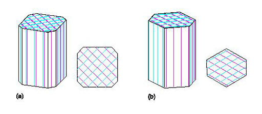
Task 3
- Look at the thin section of the amphibolite using the Virtual Microscope (found under the ‘Metamorphic rocks’ category).
Question 3.3.3
What colour are the amphibole crystals in plane-polarised light? What happens to the colour of the amphibole crystals as you rotate the thin section in View 2? What is this property called?
Answer
The amphibole crystals appear mainly grey (sometimes bluish, sometimes greenish) in plane-polarised light. When rotated, the colours change from pale grey to darker (bluish/greenish) grey: this property is pleochroism.
Question 3.3.4
See if you can locate any cleavages at about 60°, as typical of amphibole in this section. You may find this rather difficult. Can you suggest a reason for this? Look at View 1.
Answer
It can be difficult to find cleavage relationships at about 60° in thin sections when many of the amphibole crystals are in the wrong orientation (i.e. elongate in the plane of the section). To see two sets of cleavages at about 60°, it is necessary to look down the long axis of the amphibole crystal, i.e. at a basal section (see Figure 47b). In the Virtual Microscope thin section most of the amphibole crystals are aligned parallel to their long axes and both sets of cleavage planes are parallel (see also Figure 47b), but View 1 shows a typical basal section of amphibole with cleavages at about 60° (or about 120°).
3.5 Sheet silicate minerals
The sheet silicates comprise a large number of different minerals, including micas. They all share the same basic building blocks: a tetrahedral sheet (Figure 48a), and one of two kinds of octahedral sheet.
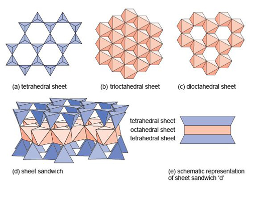
The octahedral sheets can be thought of as layers of metal hydroxides. One kind of octahedral sheet is effectively a layer of magnesium hydroxide, Mg(OH)2, where each magnesium atom is bonded to six OH groups at the corners of an octahedron. The octahedra are arranged in a plane, sharing edges, to form a trioctahedral sheet as each oxygen atom is shared between three octahedra (Figure 48b).
The other kind of octahedral sheet contains aluminium instead of magnesium, and is effectively a layer of aluminium hydroxide, Al(OH)3. In this case each oxygen atom is shared between two octahedra, hence this is a dioctahedral sheet (Figure 48c), and it leaves distinct holes in the structure. In sheet silicates, the sheets are combined to form composite structures: for example an octahedral sheet sandwiched between two tetrahedral sheets as shown in Figure 48d, and more schematically in Figure 48e.
A property common to all sheet silicate minerals is their tendency to be soft, with near-perfect cleavage parallel to the sheets. They form distinctive, platy or flake-like crystals. With (OH) groups as part of their structure, they are all hydrous minerals.
3.5.1 The mica group
Mica is a general name given to a range of sheet silicate minerals that are commonly found in igneous, metamorphic and sedimentary rocks. In igneous rocks, they crystallise from hydrous magmas with medium to high silica contents; in metamorphic rocks the parallel alignment of mica crystals defines the foliation found in slates and schists.
Micas have sandwich structures, weakly bonded by interlayer ions. Each sandwich contains a tetrahedral sheet on each side of an octahedral sheet (Figure 48d). Commonly one in four of the tetrahedra contains Al instead of Si (although the number of oxygen atoms remains unchanged), with the result that sheets have an excess negative charge. This is balanced by the presence of interlayer cations, such as K+, between the sandwiches (Figure 49a).

The bonding inside a sandwich is very strong, but between sandwiches it is very weak (due to the interlayer ions), permitting one sandwich to slide past another. Thus, mica has one perfect cleavage, parallel to the layers, so it is easy to split a mica crystal into very thin flakes (see Digital Kit).
You have seen that there are two options for making the octahedral layers: either an Al(OH)3 dioctahedral layer (Figure 48c), or a Mg(OH)2 trioctahedral layer (Figure 48b). These give rise to two important mica minerals: muscovite ('white' mica; Figure 51a), which contains dioctahedral layers, and biotite ('dark' mica; Figure 50a), which contains trioctahedral layers in which Fe2+ commonly substitutes for Mg2+.
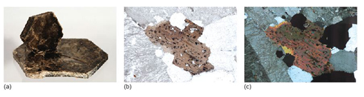
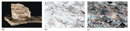
-
Why should biotite commonly be dark and muscovite be white?
-
Silicate minerals containing large amounts of Fe tend to have dark colours, and this is also true of biotite, which is often Fe rich. Muscovite contains little if any Fe, and so is usually pale coloured.
The structures of muscovite and biotite are given, in schematic form, in Figure 49a.
Micas are striking minerals under the microscope; biotites are often strongly coloured, and muscovites are colourless in plane-polarised light, but both have a perfect cleavage and vivid second- to third-order interference colours. The difference in colour between biotite, with strong pleochroism, and muscovite is diagnostic in thin section (Figures 50b and c; 51b and c). Note that basal sections show neither cleavage nor pleochroism.
3.5.2 Clay minerals
Clay minerals are stable at low temperatures and tend to form from the chemical breakdown of medium- to high-temperature aluminium-rich silicate minerals in the presence of water. Various clay minerals are produced by chemical weathering of different minerals and are commonly found in fine-grained sediments, such as mudstones and siltstones. For example, the china clay (kaolinite) of Devon and Cornwall is derived from the decomposition of K-feldspar (KAlSi3O8) in granite. Montmorillonite is formed from the breakdown of volcanic ashes. Kaolinite and montmorillonite are related to the muscovite structure, with aluminium in dioctahedral layers (Figure 49), but there is no aluminium in the tetrahedral layers. Some clay minerals (such as montmorillonite) allow water molecules to reside between their sandwich layers, which gives the clay its plasticity as the layers slide over one another.
The structure of clay minerals enables them to have a wide range of industrial and domestic applications. The large gaps between the sheets, and the large areas of the sheets, mean that many clay minerals on a fine scale readily adsorb ions and molecules onto crystal surfaces. The consequent absorbency in bulk of montmorillonite is important for its use as cat litter, and vermiculite (another clay mineral) may be used to retain moisture during seed germination. The platy structure of clays is beneficial for use in drilling muds that lubricate drill bits during drilling for crude oil.
Clays are very fine-grained, so it is difficult to observe their optical properties, even with a polarising microscope.
3.5.3 Other sheet silicates
Some other sheet silicates that you are likely to meet include talc, chlorite and serpentine. These minerals have structures related to biotite, with magnesium (and iron) in trioctahedral layers (as summarised in the right-hand column of Figure 49). Unlike biotite, however, their tetrahedral layers contain no aluminium, only silicon. These layers, therefore, have no net electrical charge, and so no interlayer ions are required to balance charges. Without the interlayer ions, there is little to hold the layers together.
-
How would you expect the hardness of talc to compare with that of biotite?
-
Without interlayer ions between the sandwich layers, minerals such as talc are much softer than biotite. Talc is one of the softest minerals known, with a hardness of 1 on Mohs' scale (Table 2).
All of these minerals are stable at low temperatures (and up to surprisingly high pressures) and tend to form (serpentine, especially) by the breakdown of high-temperature Mg-rich minerals, such as olivine (Mg2SiO4), under hydrous conditions. These minerals, therefore, contain hydroxyl groups and are common (serpentine and talc, especially) in basaltic and mantle rocks that have been altered by watery fluids. Chlorite is common in many low-temperature metamorphic rocks derived from sediments and from basaltic igneous rocks.
Pyrophyllite, with dioctahedral layers (Figure 49b), is a low-temperature metamorphic mineral found in aluminium-rich sedimentary rocks such as slates.
Activity 3.4 Micas in hand specimen and thin section
Task 1
This activity will help you to recognise micas in hand specimen and thin section.
For this activity you will require the muscovite mica sheet, granite and schist in the Digital Kit and the Virtual Microscope.
- Examine the thin flake cleaved from a larger crystal of muscovite mica in the Digital Kit. The fact that it is easy to separate such flat crystal flakes (see also the video clip of a peeling flake of muscovite mica in the Digital Kit) indicates that mica has an excellent cleavage.
- Examine the granite in the Digital Kit. This contains small elongate crystals of dark mica (biotite), which appear to glint in the light as the specimen is rotated. If you zoom in using the Digital Kit to look at these crystals more closely, you may be able to make out flat cleavage surfaces.
- Compare the granite (which contains biotite) with the schist. The silvery mineral in the schist is the white mica, muscovite.
- Examine the granite in thin section using the Virtual Microscope (found under the ‘Igneous rocks’ category) in plane-polarised light. The brown crystals (View 1, especially) are biotite.
Question 3.4.1
What happens to the colour of the biotite crystals in PPL when you rotate the stage (View 1)? What is this property called?
Answer
The colour of the biotite crystals changes from pale brown to dark reddish-brown as they are rotated. This property is pleochroism.
Task 2
- Note that the biotite crystals contain tiny, dark 'haloes' (often referred to as pleochroic haloes) surrounding minute specks (tiny inclusions). Now examine the biotite crystals between crossed polars and as you rotate the thin section.
Question 3.4.2
How do the haloes behave as you rotate the XP view (View 1)?
Answer
You should find that the haloes around inclusions in the biotite always appear dark between crossed polars, whereas normal biotite shows interference colours, although they are often masked by the strong colour of biotite. The haloes are actually regions of biotite that have been damaged by radiation, becoming amorphous (and optically isotropic). The radiation comes from the minute crystals at the centre of every halo: most of these are the radioactive mineral, zircon (ZrSiO4), that contains minor amounts of uranium.
Task 3
- Examine the schist (a metamorphic rock) in plane-polarised light, then between crossed polars. You should find curved, sheaf-like masses (View 2, especially) that show colourful, high-order interference colours. These are crystals of white mica (muscovite).
3.6 Framework silicates
Framework silicates are the most abundant silicates in the Earth's crust. They have complex crystal structures, with each SiO4 tetrahedron joined to four others, producing a three-dimensional framework. In feldspars, some of the silicon atoms are replaced by aluminium, and singly charged cations (e.g. Na+ or K+) are required to maintain charge balance.
3.6.1 Silica minerals
The silica minerals have fully polymerised structures and are essentially pure silica. There are several minerals with the chemical formula SiO2, although most of them are usually referred to as quartz, as it is difficult to recognise the differences between them in both hand specimen and thin section. The SiO2 phase diagram (Figure 52) illustrates that at least five forms of SiO2 can be found in the Earth's crust and a further high-pressure form called stishovite is stable at pressures greater than 7.5 GPa. At progressively higher pressures, the Si and O atoms are packed closer together so that coesite is denser than α-quartz and stishovite is denser than coesite. Silica minerals are very common in sedimentary, igneous and metamorphic rocks because they are chemically and mechanically stable under a wide range of conditions. Figure 52 can be used to predict which forms of SiO2 are found in different rocks: α-quartz is found in sedimentary rocks whereas β-quartz is found in high-temperature/low-pressure metamorphic rocks. Coesite is a characteristic mineral of some high-pressure metamorphic rocks whereas stishovite has only ever been discovered in nature in meteorite impact sites where very high pressures and temperatures were developed. In igneous rocks, tridymite and cristobalite are restricted to lavas that crystallised rapidly from high-temperature silica-rich magmas.
SAQ 7
What pressure would be required to convert silica into stishovite at 300 °C?
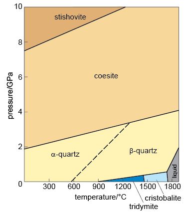
The strong, three-dimensional bonding in quartz, which is dominantly covalent on account of there being no metal cations present, means that there are no definite planes of weakness and, therefore, no cleavage. So, when broken, quartz shatters to form glassy fragments with a curved, conchoidal fracture. The strong bonding also makes quartz very hard and extremely resistant to chemical attack. Consequently, quartz grains can survive transport by wind or water over vast distances, eventually being deposited as sand grains.
Although quartz is very pure SiO2, it can sometimes contain small amounts of impurities such as aluminium, iron, lithium and titanium. The effect of these impurities is to produce quite dramatic colours in what would otherwise be an entirely colourless mineral (Figures 7 and 53a).

Under the microscope, quartz lacks cleavage and colour and has low first-order, grey-white interference colours (Figure 53b and c). Being chemically stable, quartz crystals look clean compared with feldspars, which are almost always turbid or cloudy.
Activity 3.5 Quartz in hand specimen and thin section
This activity will help you to recognise quartz in hand specimen and thin section. For this activity you will need to look at quartz and granite in the Digital Kit and granite in the Virtual Microscope.
Although quartz crystals can grow to form large, well-developed single crystals (such as the well-formed crystals shown in the Digital Kit), it is more common to find quartz crystals as irregular-shaped grains in rocks, often filling the gaps between other crystals.
- Examine the granite sample, and particularly the close-up image in the Digital Kit. This contains dark mica crystals (biotite) plus a white mineral. It also contains grey/glassy grains, which are quartz crystals. Note that they have no cleavage.
- Look at the granite in thin section using the Virtual Microscope (found under the ‘Igneous rocks’ category) in plane-polarised light. The quartz crystals have very low relief, and are almost invisible. When viewed between crossed polars they show low-order, grey interference colours and, unlike the other low-relief mineral in the thin section, they do not feature any regular kind of patterning indicative of twinning (see Activities 3.6 and 3.7).
- When viewed between crossed polars, some of the quartz crystals, such as the one featured in View 4, do not snap in and out of extinction as uniformly as other minerals in the thin section. Instead, they show undulose or 'wavy' extinction, whereby different parts of a crystal are in extinction at slightly different positions from other parts (see also coordinates 2400,800). This effect is because the structures of different regions of the crystal are slightly out of alignment with each other, due to the quartz crystal lattices having been stressed. This is especially common in metamorphic rocks, but can occur in other rocks that either contain relict crystals (reflecting an earlier history), or have been deformed after formation.
3.6.2 Feldspars
Feldspars are especially common minerals and make up about 60% of the Earth's crust. They crystallise from a wide spectrum of magmas and are found in many metamorphic and sedimentary rocks. The name 'feldspar' refers to a group of silicate minerals that share the same basic structure. The three most important feldspar minerals are orthoclase (KAlSi3O8), albite (NaAlSi3O8) and anorthite (CaAl2Si2O8).
At high temperatures there is complete solid solution between orthoclase and albite, as K and Na substitute for each other (in the same way that Fe and Mg substitute for each other in olivine). Feldspars with compositions within this range are called alkali feldspars. At lower temperatures the alkali feldspar solid solution is not complete, and if an alkali feldspar crystal of an intermediate composition (e.g. Na0.3K0.7AlSi3O8) were cooled very slowly, it would 'unmix' into Na-rich and K-rich phases - a process known as exsolution (meaning 'from solution'). The result is a crystal mainly of one composition (K-rich), containing streaks of another composition (Na-rich), producing what is known as perthitic texture (particularly noticeable in thin section when viewed between crossed polars). You will see examples of perthitic texture in Figure 54 and Activity 3.7.
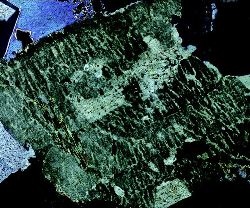
There is also complete solid solution between albite and anorthite at high and intermediate temperatures: these are the plagioclase feldspars. Plagioclase feldspars crystallise from a range of magma compositions, depending on the proportion of Ca and Na available. Solid solution in plagioclase feldspars is rather more complex than in alkali feldspars, because Na+ and Ca2+ have different charges. A coupled substitution is required to maintain charge balance whereby two substitutions occur simultaneously:
Na+ substitutes for Ca2+and Si4+ substitutes for Al3+
This coupled substitution is more usually written as:
Na+ + Si4+![]() Ca2+ + Al3+
Ca2+ + Al3+
There is no solid solution between KAlSi3O8 and CaAl2Si2O8 because of the large size difference between K+ and Ca2+ (about 30%). Ionic substitution is, therefore, not possible.
The overall compositional range of feldspars can be shown on a ternary diagram (Figure 55). Ternary diagrams are very useful tools in geology, and you will meet them again later in the course. Their use is explained in Box 4.
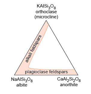
Box 4 Ternary diagrams
A ternary diagram can be used to plot the composition of a mineral (or indeed, any multi-component substance or mixture) in terms of three end-member components (A, B and C). The diagram consists of a triangle, with each corner representing one of the three end members (100% A, 100% B or 100% C) (Figure 56a).
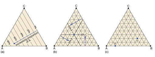
To plot a mineral's composition, you need to represent the proportion of each component. In Figure 56a, different proportions of component A are represented by lines parallel to the edge BC (0% A). Likewise, different proportions of component B would be represented by lines parallel to the edge CA (0% B), and so on.
To plot a mineral whose composition is: 40% A, 30% B and 30% C, you:
- determine on which 'A' line the 40% composition must lie (as in Figure 56a and b)
- find the 30% 'B' line (Figure 56b).
The intersection of these two lines at a point marks the composition of the mineral.
As a final check, you can identify the 'C' line, which should pass through the same point (Figure 56b).
SAQ 8
Using the ABC ternary diagram in Figure 56c, determine the compositions indicated by the two points X and Y.
Twinning in feldspar
You were introduced to twinning in Section 1.5. The presence of twinning is a common feature of feldspars and can be a useful diagnostic property.
-
Look at the twinned orthoclase feldspar in Figure 57a. With reference to the schematic above the specimen, you should be able to see that the crystal is twinned. How are the two twin components related?
-
The crystal appears to be made of two parts, which look very similar when viewed from different directions - and yet they seem 'squashed' together. These are twin components that overlap with each other (they are said to be inter-penetrant) and are related by a 180° rotation along the long (z) axis of the crystal (Figure 57a).
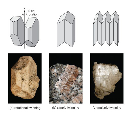
This crystal is a kind of growth twin, called a Carlsbad twin, which is especially common in K-feldspar. The two twin domains are related by a 180° rotation (Figure 57a). Twinning in feldspars does not have to be inter-penetrant and other types of twinning may occur by reflection along twin planes, producing either simple or multiple twinning (Figure 57b and c).
How might the feldspars be distinguished? In plane-polarised light, feldspars have low relief and are colourless. Both alkali and plagioclase feldspars are susceptible (though not necessarily under the same conditions) to alteration to fine-grained micas and clay minerals, which often gives them a turbid (dirty-looking) appearance (e.g. Figure 58b). However, both plagioclase and alkali feldspars have some distinctive features under the microscope.
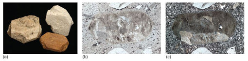
-
Would you expect to be able to see simple twinning in a thin section of a feldspar when viewed with plane-polarised light?
-
Not normally. There is unlikely to be a significant difference in colour or relief between the two twin components.
-
What would happen if the section were viewed between crossed polars?
-
On either side of the twin boundary, the crystal orientations would be different. Therefore the adjacent twin domains would go into extinction at different times. As the microscope stage was rotated, first one half of the twin would go into extinction, then the other half (e.g. Figure 58c).
Twinning in feldspars is most obvious between crossed polars. In addition to simple twins, plagioclase feldspar often shows repeated or multiple twinning (Figures 57c and 59a) usually on a microscopic scale, which gives crystals a striped appearance (Figure 59c). This is often referred to as lamellar twinning and is a characteristic feature of plagioclase feldspars.
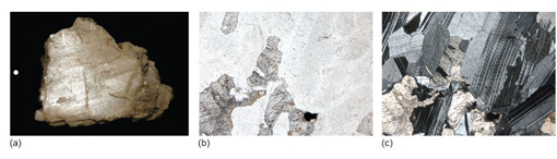
One variety of K-feldspar, known as microcline, shows two kinds of repeated twinning in thin section, with one set of twins arranged at 90° to the other set. The lamellar twins overlap each other and have 'fuzzy' edges, giving a 'tartan' appearance known as cross-hatched twinning (see Figure 60).
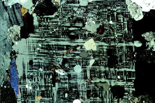
Activity 3.6 Simple twinning in orthoclase feldspar
This activity will help you to recognise orthoclase feldspar in hand specimen and thin section.
For this activity you will need the Digital Kit and the Virtual Microscope.
- The orthoclase mineral samples shown in the Digital Kit (see Feldspar (orthoclase) - 'Twinned crystals') show interpenetrant twins. The rotating specimen in the movie is particularly useful to gain a better understanding of the manner in which the crystals have intergrown.
- The pink phenocrysts of orthoclase feldspar are particularly striking in the granite rock specimen of the Digital Kit. Go to the orthoclase crystal granite in the Digital Kit ('Phenocryst in granite') and look at the broken surface. Can you see any flat, reflective surfaces? These are cleavage surfaces. In the Digital Kit, a reflective cleavage surface is visible in the matching image ('Twinning in phenocryst'). Cleavage directions differ on each side of the twin plane that runs down the middle of the crystal. This is a simple twin.
- Now look at the full-section view of the porphyritic rhyolite thin section using the Virtual Microscope (found under the ‘Igneous rocks’ category). In thin section you should see some large, cloudy, or turbid, crystals. These are orthoclase feldspar. Feldspars are often turbid like this, because of alteration - this provides a way of distinguishing feldspars from quartz, which forms the large, clear, colourless crystals, a few of which have faces at 120° in this thin section. Look under low power at the field of view centred at coordinates 3800,1300, using plane-polarised light, so that you can see the difference between the clear, low-relief quartz, and the turbid feldspar crystals.
- Now observe this view between crossed polars. Note that some of the feldspar crystals appear to be divided into two parts. In View 1, at the very edge of the field of view between crossed polars, you can see there is a straight-line division between two parts of the feldspar crystal that go into extinction in different positions. This is a twin plane, and the crystal is a simple twin; the two parts are in slightly different orientations to each other (Figure 58c).
Activity 3.7 Multiple twinning in feldspar
This activity will help you to recognise plagioclase and microcline feldspars in thin section. For this activity you will need to view plagioclase feldspar in the Digital Kit and the diorite and granite thin sections using the Virtual Microscope (both of which can be found under the ‘Igneous rocks’ category).
- Examine the rotation video clip of plagioclase feldspar in the Digital Kit and note that reflecting parallel stripes become visible briefly as the crystal is rotated (at about 80-95°). These reflections are the result of multiple twinning. This effect is not very commonly seen in hand specimen, but is very common in thin section as demonstrated below.
- Examine the diorite thin section at low magnification between crossed polars. You should see that a lot of crystals show regular dark and light stripes (like a 'zebra' crossing). These crystals are plagioclase feldspar, and they contain multiple twins - with twin planes developed in only one direction. This kind of twinning is lamellar twinning. Lamellar twinning (Figure 59c) is characteristic of plagioclase feldspar, and provides a good way of identifying this mineral in thin section.
- Now examine the granite thin section. You should find a mineral that shows a rather diffuse grid-like pattern when viewed between crossed polars (View 2). This mineral is a type of K-feldspar called microcline, distinctively showing two sets of multiple twins, developed at right angles to each other. This is called cross-hatched (or 'tartan') twinning (Figure 60).
Activity 3.8 Zoning in plagioclase
This activity will help you to recognise compositional zoning of crystals as developed in plagioclase feldspar. For this activity you will need to view the granite thin section using the Virtual Microscope.
The extinction angle of plagioclase varies with its composition. In crystals that vary in composition from core to rim (not uncommon in plagioclase), it produces a distinctive effect when crystals are viewed between crossed polars.
Examine the granite thin section between crossed polars. In View 3, on rotation, the plagioclase crystal shows varying extinction between a central zone and a marginal zone. This effect is due to progressive compositional variation, often called zoning, which may arise due to mineral growth or to diffusion of elements (as in olivines). In this case, when the rotation is at about 65° it is possible to see 'ghosts' of crystal faces, indicating growth zoning and the development in stages of a well-shaped crystal until it finally filled in the remaining space. Strongly developed concentric zoning can often be a distinctive feature of plagioclase.
In coloured minerals, zoning can show up as concentric colour banding. This is a feature of some pyroxenes.
3.7 Non-silicate minerals
3.7.1 Carbonates
The most common carbonate mineral is calcite (CaCO3) (Figure 61a). Calcite is one polymorph of CaCO3. Another polymorph is aragonite, which has a different crystal structure - it is orthorhombic rather than trigonal. Aragonite is less stable than calcite under ambient conditions. Many marine organisms initially build their skeletons of aragonite but, when they die, their shells drop to the sea floor and gradually the aragonite transforms into calcite.
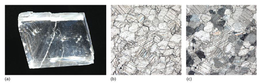
Calcite is the major constituent of limestone rocks. Limestones are important industrial minerals; they are used not only as aggregates in the construction industry and in powdered form as filler for plastics, paints and rubber, but also as a major constituent of cement.
In thin section, calcite is distinctive: it is a highly anisotropic mineral, with high-order interference colours (Figure 61c). In hand specimen it is quite a soft mineral (hardness 3 on Mohs' scale, Table 2) and has three excellent cleavages (Figure 61a). Dilute (5-10%) hydrochloric acid (HCl) provides a good test for calcium carbonate in hand specimen. A few drops, carefully applied, will fizz, giving off carbon dioxide:
Dolomite (CaMg(CO3)2) is another carbonate mineral that is found in many limestones. Dolomite rocks form when there is an excess of Mg ions available, either during their formation or during later burial.
3.7.2 Oxides
Oxides are an important group of non-silicate minerals. Hematite (Fe2O3) and magnetite (Fe3O4) are the two most common oxides of iron. Hematite contains iron in its most oxidised form (Fe3+) and often has a striking red-brown colour similar to rust (hydrated iron oxide) and is responsible for the intense red colour of some desert sandstones. Magnetite and hematite are found in banded iron formation deposits of Precambrian age which are the main sources of iron ore today (Figure 62). In most rocks, they are present only as accessory minerals.
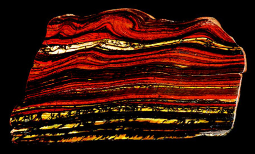
Magnetite is a member of the spinel group of minerals, which have the general formula AB2O4, where A represents 2+ cations and B represents 3+ cations. A large number of elements can substitute into the spinel structure so that spinel group minerals are present in a wide range of igneous, metamorphic and sedimentary rocks. Chromite (FeCr2O4) is a chrome spinel found in silica-poor igneous rocks and is an important source of chromium.
-
Both hematite and magnetite are opaque minerals. How would you expect them to appear in plane-polarised light and between crossed polars?
-
Opaque minerals appear black both in plane-polarised light and between crossed polars, which makes specific identification difficult. By contrast, non-opaque isotropic minerals are black only when between crossed polars - which is an important distinction.
3.7.3 Sulfides
Sulfur is an essential constituent of sulfide minerals, in which it commonly bonds with metals such as copper, lead and zinc. Sulfides can be important economically when they are concentrated in mineral deposits. They often occur as vein mineralisation, deposited by hot, watery fluids passing through fractures, fault zones and permeable rocks. Some are formed by segregation processes in sulfur-rich magmatic systems. Mining followed by smelting of the sulfide minerals allows the metals to be extracted. Examples of economically important sulfide mineral deposits include the Pb-Zn deposits of the Mississippi Valley and the vast disseminated Cu deposits of the Andes.
Pyrite (FeS2) (Figure 63a) is the most commonly encountered sulfide mineral in vein deposits and is also found in igneous, metamorphic and sedimentary rocks. Other common sulfide minerals in vein deposits include galena (PbS) (Figure 63b), sphalerite (ZnS) (Figure 15c) and chalcopyrite (CuFeS2).
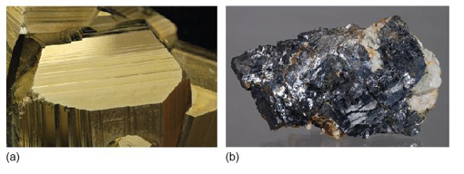
3.8 Summary of Section 3
- The most important rock-forming minerals on Earth are silicate minerals, composed of silicon, oxygen and a variety of metal cations. The basic building block of silicate minerals is the SiO4 tetrahedron. However, what defines the structural variety and with it a range of properties of silicate minerals is the ability of SiO4 tetrahedra to link together, or polymerise, by sharing oxygen atoms in different ways and in different proportions. Increasing polymerisation increases the silicon to oxygen ratio to reach that of quartz, which has a fully polymerised structure.
- Silicate mineral groups are built of different forms of three-dimensional structure: isolated units, chains, sheets and frameworks, with a corresponding increase in the silicon to oxygen ratio from 1 : 4 to 1 : 2. These three-dimensional structures are mostly bound together by metal cations. The crystal structures of these mineral groups have important consequences for the physical properties of the minerals.
- The main silicate mineral groups covered in this section, for which the chemistry, structure, occurrence and properties are considered, are those with isolated SiO4 tetrahedra (olivine and garnet), the chain silicates (pyroxene and amphibole), the sheet silicates (micas and clay minerals) and the framework silicates (quartz and feldspar).
- Major non-silicate mineral groups include the carbonates, oxides and sulfides. Carbonates are an important part of the carbon cycle whereby carbonate minerals are precipitated from seawater, often as skeletons of organisms, and deposited on the sea floor. Oxide and sulfide minerals can be economically important as sources of metals when they are concentrated as mineral deposits.
3.9 Learning outcomes for Section 3
Now you have completed this section, you should be able to:
- summarise the range of silicate mineral structures in terms of various degrees of SiO4 polymerisation
- outline the essential structural features of the common rock-forming minerals: olivine, garnet, pyroxene, amphibole, mica, quartz and feldspar
- give examples of some physical properties of minerals that can be attributed to specific crystal structural features
- describe the basic chemistry and properties of common rock-forming minerals in the Digital Kit
- describe the distinguishing features of the major rock-forming minerals in hand specimen and thin section.
Now try the following questions to test your understanding of Section 3.
SAQ 9
The structure of quartz is built entirely of SiO4 units. Why, then, is its chemical formula SiO2?
SAQ 10
Quartz and mica are both silicate minerals, but they have very different cleavage properties. How do quartz and mica differ in this respect, and why?
SAQ 11
What is meant by solid solution? Give two examples of important rock-forming minerals that exhibit solid solution.
Conclusion
By studying this course you have been introduced to the most common technique used by geologists to study minerals in rocks in order to understand geological processes such as rock formation, rock deformation, weathering and metamorphism. It's a science known as mineralogy. Mineral composition, structure and microtextures all contain clues to the processes of rock formation, and the recognition, identification and classification of minerals is a key skill for geologists.
This course should have helped you to understand the background to mineral formation, recognition and classification, and introduced the use of the polarising microscope, a tool that still forms the bedrock of many geological investigations. Activities using the microscope, delivered using a virtual microscope system, provided the opportunity to acquire some of the core skills for any further geology studies.
If you'd like an interactive overview of the geological makeup of the landscape of the British Isles, take a look at our Geology Toolkit.
Keep on learning

Study another free course
There are more than 800 courses on OpenLearn for you to choose from on a range of subjects.
Find out more about all our free courses.
Take your studies further
Find out more about studying with The Open University by visiting our online prospectus.
If you are new to university study, you may be interested in our Access Courses or Certificates.
What's new from OpenLearn?
Sign up to our newsletter or view a sample.
For reference, full URLs to pages listed above:
OpenLearn - www.open.edu/ openlearn/ free-courses
Visiting our online prospectus - www.open.ac.uk/ courses
Access Courses - www.open.ac.uk/ courses/ do-it/ access
Certificates - www.open.ac.uk/ courses/ certificates-he
Newsletter - www.open.edu/ openlearn/ about-openlearn/ subscribe-the-openlearn-newsletter
Acknowledgements
This course was written by Simon Kelley.
Except for third party materials and otherwise stated (see terms and conditions), this content is made available under a Creative Commons Attribution-NonCommercial-ShareAlike 4.0 Licence.
Course image: Alan Colson in Flickr made available under Creative Commons Attribution-NonCommercial-ShareAlike 2.0 Licence.
The material acknowledged below is Proprietary and used under licence (not subject to Creative Commons Licence). Grateful acknowledgement is made to the following sources for permission to reproduce material in this course:
Figures 2, 10b: Peter Sheldon.
Figures 5, 7, 9, 10a, c, d, 11a, b, 14c, 15c, 17c, 19d, 29b, 30, 35, 36, 39, 43, 44, 45, 46, 50, 51, 53, 54, 57, 58, 59, 60, 61, 62, 63: Andy Tindle.
Figure 11: © Joel Arem/Science Photo Library.
Every effort has been made to contact copyright owners. If any have been inadvertently overlooked, the publishers will be pleased to make the necessary arrangements at the first opportunity.
Don't miss out:
If reading this text has inspired you to learn more, you may be interested in joining the millions of people who discover our free learning resources and qualifications by visiting The Open University - www.open.edu/ openlearn/ free-courses