
1.5 Basic principles
The basic principles underlying the FEM are relatively simple. Consider a body or engineering component through which the distribution of a field variable, e.g. displacement or stress, is required. Examples could be a component under load, temperatures subject to a heat input, etc. The body, i.e. a one-, two- or three-dimensional solid, is modelled as being hypothetically subdivided into an assembly of small parts called elements – ‘finite elements’. The word ‘finite’ is used to describe the limited, or finite, number of degrees of freedom used to model the behaviour of each element. The elements are assumed to be connected to one another, but only at interconnected joints, known as nodes . It is important to note that the elements are notionally small regions, not separate entities like bricks, and there are no cracks or surfaces between them. (There are systems available that do model materials and structures comprising actual discrete elements such as real masonry bricks, particle mixes, grains of sand, etc., but these are outside the scope of this course.)
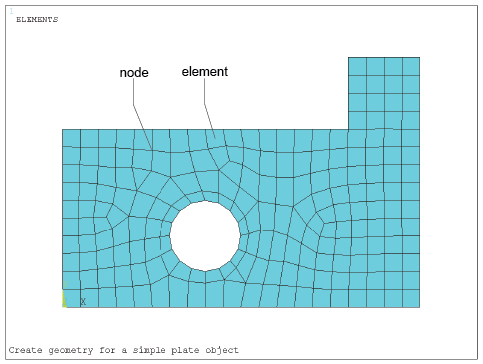
The complete set, or assemblage of elements, is known as a mesh . The process of representing a component as an assemblage of finite elements, known as discretisation, is the first of many key steps in understanding the FEM of analysis. An example is illustrated in Figure 1. This is a plate-type component modelled with a number of mostly rectangular(ish) elements with a uniform thickness (into the page or screen) that could be, say, 2 mm.
The field variable, e.g. temperature, is probably described throughout the body by a set of partial differential equations that are impossible to solve mathematically. Instead, we assume that the variable acts through or over each element in a predefined manner – another key step in understanding the method. This assumed variation may be, for example, a constant, a linear, a quadratic or a higher order function distribution. This may seem to be a bit of a liberty, but it can be surprisingly close to reality.