
1.7 Hints and tips on finite element analysis
Don’t rely on one run. Refine the mesh in areas of high stress, repeat two or three times, check the iteration effects.
Remember that we are only ever solving a model of the real problem.
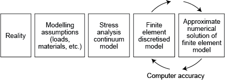
A good finite element model, once set up, is about a 95% accurate solution of the field equations, which themselves are based on a theoretical model, which is idealised from reality, and which uses assumed material properties (Figure 3).
Don’t confuse the processing accuracy of the computer with the validity of the solution.
Computer-aided FEA makes a good engineer better – it makes a bad engineer dangerous !
Finite element model solution (outline)
Here is a reminder of the main steps involved in the FEA of a structural problem.
Pre-processing stage
The component under investigation is ‘discretised’ into an assembly of finite elements in the prerocessing stage, with particular reference to the following six aspects.
- Element boundaries should coincide with structural discontinuities.
- Points of application of forces (and restraints) must coincide with suitable nodes, and any abrupt changes in distributed loading must occur at element boundaries. (Pressures are applied to the centroids of element faces.)
- Nodes should be at the points of interest for which output data are required, e.g. displacements, reaction forces, etc.
- The selection of element order (e.g. linear, parabolic, cubic) defines the interpolation or shape function of displacements between nodal points, i.e. the order of a polynomial in x , y and z directions, and hence the variation of stress/strain. Furthermore, the element type (e.g. spring, rod, beam, triangular and quadrilateral planar or shell, tetrahedral or hexahedral (brick) element) needs to be chosen. Often, the expected behaviour and physical shape of the component being analysed will guide the selection.
- Boundary conditions (e.g. applied loads, fixed nodes and restraints) and material properties must be entered. Loads and restraints are often the most difficult parameters to represent accurately, and have a significant influence on the predictions.
- Extensive model checks for cohesiveness, clashes, ‘cracks’, aspect ratios of elements, etc., must be carried out.
Solution stage
The fundamental unknowns to be solved are displacements u , v and, for fully three-dimensional analysis, w , for each node, with reference to a global frame of reference. Other data such as stresses and restraint reaction forces are calculated from these solution displacements, via the strains, at a later stage in the computation.
Within each element, a set of virtual displacements is applied and expressed in terms of the unknown displacements of the nodes. An element stiffness matrix is formulated using a numerical integration technique on the basis that actual displacements occurring will be those that minimise the strain energy. (This minimising of a functional parameter as a convergence criteria is an example of the calculus of variations.)
The individual element stiffness matrices are then combined to form a global stiffness matrix for the whole body from which a vast field of linear algebraic equations relating nodal forces, element stiffnesses and nodal displacements are formed. Boundary conditions are applied to the relevant nodes and the displacements and are then solved using numerical techniques such as Gaussian elimination, Gauss–Seidel iteration or Cholesky square root methods. For each node connecting two or more elements, compatibility of displacements and equilibrium of forces are maintained at that node (although derivatives of the displacement interpolations generally are not continuous across interelement boundaries). The assembly of the global stiffness matrix and the solution of the displacement equations occupies most of the processing time.
Once a solution for the nodal displacements has been obtained (or in the case of iterative techniques, once satisfactory convergence is achieved for them all) for each element, the stresses are computed based on the material data entered, the original element dimensions and newly computed nodal displacements.
Post-processing stage
The results of the solution are given in the form of stress plots (e.g. maximum principal, minimum principal, maximum shear, von Mises), deformed geometry (i.e. the distorted shape) and listings of nodal displacements ( u x , u y , u z ). Picture files can be created to obtain hard copies, or individual programs written to read the results file and carry out further data processing, if required.