Interactive step-by-step solution

1. Specify title
   • Specify a title for your project.
2. Define parameters to be used for geometry input
   • HEIGHT = 0.20
   • WIDTH = 0.50
   • RADIUS = 0.10
   • THICK=0.01
3. Set preferences
   • Make sure that Structural Analysis option is enabled.
4. Define element types
   • Choose an 8-node 1PLANE element (PLANE183).
5. Define options for your element types
   • Set the element options so that it behaves as ‘plane stress with thickness’.
   • The thickness of the element should be set to 0.01.
6. Define material properties

   Set material properties to:

   • Young’s modulus: 2.07 × 10 ¹¹
   • Poisson’s ratio: 0.29
7. Create rectangular area
   • Create a rectangular area with

     Width = WIDTH

     Height = HEIGHT

8. Create circular area
   • Create a circular area with centre at (0, 0) and Radius = RADIUS
9. Subtract hole from plate
   • Use Bollean operations to subtract the hole from the rectangle.
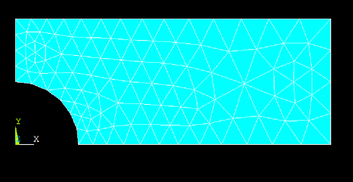
10. Mesh the area with a default mesh
    • Choose ‘Triangular elements’ for Shape.
    • Click Mesh.

    In this example we choose to mesh with triangular elements.

    It should look something like this:

    

    Figure 4 Diagram showing a quarter of the plate with rather large triangular meshing elements

    Show description|Hide description

    The figure shows a coarse meshing of the quarter plate. It is a rectangular shape with a quarter circle cut away from the bottom left corner, representing the quarter of the circular hole. The plate is meshed with about 45 large triangular elements. This represents about seven triangles per long side and three per short side. The triangles are smaller near the cut area.

    Figure 4 Diagram showing a quarter of the plate with rather large triangular meshing elements
11. Apply displacement constraints

    The boundary conditions we apply must represent the symmetric nature of the problem.

    Note: we are going to do this in two distinct steps as an illustration of applying a simple fixed displacement to the nodes attached to a line. In this case, however, as the displacements are equal, i.e. zero, we could have done this in a single step.

    • Apply structural displacement BC to the left edge of the model.
    • Pick UX (x- direction displacement).
    • Enter 0 for Displacement Value.
    • Apply structural displacement BC to the bottom edge of the model.
    • Pick UY (y-direction of the displacement).
    • Enter 0 for Displacement Value.

    Alternative route:

    You can achieve the same result by applying a symmetry boundary condition on left-most and bottom edges.

12. Apply pressure load

    The unit pressure load will be applied to the line at the right.

    • Apply a structural pressure load right-hand edge (line 2).
    • Enter –1.0 for ‘Load Pressure’ value (this ensures that the pressure is outwards as we have a tensile load).
13. Solve
    • Solve the arrangement.
14. Plot the deformed shape
    • The maximum displacement is given as DMX = 0.321 × 10–11. This seems reasonable for a unit load.
15. Plot the element stress in the x direction

    The element stress is a good thing to look at after the displacement. It will show us any steep gradients.

    Note that we have rather steep gradients in the area of concern around the hole.

    We will address this by refining the mesh.

16. Refine mesh

    This command will subdivide all the elements.

    However, in some programs before refining the mesh we need to remove the loads.

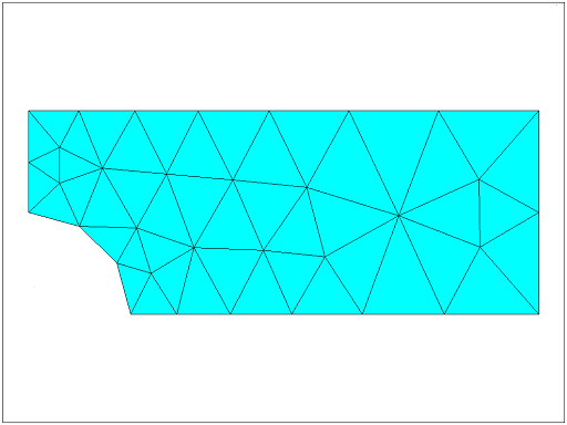
    The resultant global refinement is given below. Compare this mesh with the one above.

    

    Figure 5 The same plate as the one shown in Figure 4 but with finer meshing.

    Show description|Hide description

    This figure shows the same plate as in Figure 4, however with much smaller elements. This time there are about 14 triangles per long side and about four per short side. On average the area of each of these elements is about one quarter of the area of elements shown in Figure 4.

    Figure 5 The same plate as the one shown in Figure 4 but with finer meshing.
17. Refine mesh near hole

    You should refine further around the top of the hole.

    • Select the three nodes at the top tip of the circular cut.
    • Refine the mesh in these elements/nodes.

    This produces more elements in the area of interest.

18. Re-introduce loads and Solve

    Repeat steps 11 and 12 above to add load, then solve.

19. Read in the new data set and plot the element stress in the x-direction
    • Choose X-Component of stress to plot.

    The stress contours are now smoother across the element boundaries and the stress legend shows a maximum value of 4.39 Pa. We must check these results. Find the theoretical stress concentration factor, K _t , for this problem in any good source. We determine that for this geometry, K _t = 2.17. The maximum stress is given by:

    ( K _t )(load)/(net cross sectional area)

    Using a pressure of p = 1.0 Pa we get:

    σ _{x, MAX} = 2.17× p ×(0.4)(0.01)/[(0.4-0.2)*0.01] = 4.34

    The computed maximum value is 4.38 Pa which is less than 1% in error, assuming that the value of K _t is exact.

20. Exit the program.