
1.2 The median
Despite the variability in the data, Table 1 does provide some idea of the price you would expect to pay for a 100 g jar of that particular instant coffee in the Milton Keynes area on that particular day. The information provided by the batch can be seen more clearly when drawn as a stemplot, shown in Figure 1 of Example 2.
Example 2 Picturing the coffee data
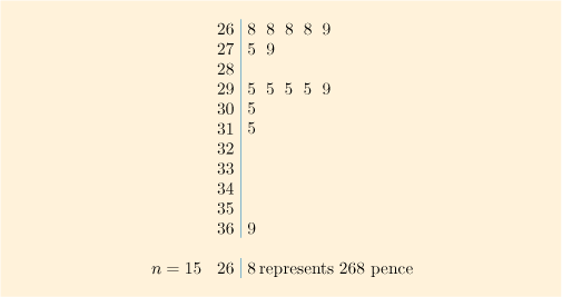
This stemplot shows at a glance that if you shop around, you might well find this brand of coffee on sale at less than 270p. (Indeed some stores seem to have been ‘price matching’ at the lowest price of 268p.) On the other hand, if you are not too careful about making price comparisons then you might pay considerably more than 300p (£3). However, you are most likely to find a shop with the coffee priced between about 270p and 300p. Although there is no one price for this coffee, it seems reasonable to say that the overall location of the price is a bit less than 300p.
The median of the batch is a useful measure of the overall location of the values in a batch. It is defined as the middle value of a batch of figures when the values are placed in order. Let us examine in more detail what that means.
The stemplot in Figure 1 shows the prices arranged in order of size. We can label each of these 15 prices with a symbol indicating where it comes in the ordered batch. A convenient way of showing this is to write each value as the symbol plus a subscript number in brackets, where the subscript number shows the position of that value within the ordered batch. Figure 2 shows the 15 prices written out in ascending order using this subscript notation.
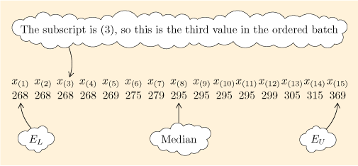
The lower extreme, , is labelled and the upper extreme, , is labelled . The middle value is the value labelled since there are as many values, namely 7, above the value of as there are below it. (This is not strictly true here, since the values of , and happen also to be actually equal to the median.)
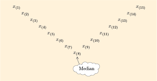
This is illustrated in Figure 3 by a V-shaped formation. The median is the middle value, so it lies at the bottom of the V. (This way of picturing a batch will be developed further in Subsection 3.2.)
If you wanted to make a more explicit statement, then you could write: The median price of this batch of 15 prices is 295p.
If we picture any batch of data as a V-shape like Figure 3, the median of the batch will always lie at the bottom of the V. In the ordered batch, it is more places away from the extremes than any other value.
In general, the median is the value of the middle item when all the items of the batch are arranged in order. For a batch size , the position of the middle value is . For example, when , this gives a position of , indicating that is the median value. When is an even number, the middle position is not a whole number and the median is the average of the two numbers either side of it. For example, when , the median position is , indicating that the median value is taken as halfway between and .
Example 3 uses prices of a digital camera to illustrate how the median is found for an even number of values.
Example 3 Digital cameras
Table 2 shows prices for a particular model of digital camera as given on a price comparison website in March 2012.
60 |
70 |
53 |
81 |
74 |
85 |
90 |
79 |
65 |
70 |
If we put these prices in order and arrange them in a V-shape, they look like Figure 4.
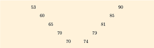
Because 10 is an even number, there is no single middle value in this batch: the position of the middle item is . The two values closest to the middle are those shown at the bottom of the V: and . Their average is 72, so we say that the median price of this batch of camera prices is £72.
The following activity asks you to find the median for an even number of values, using a stemplot of prices for small flat-screen televisions.
Activity 1 Small flat-screen televisions
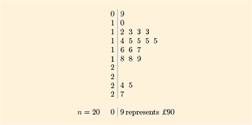
Figure 5 is a stemplot of data on the prices of small flat-screen televisions. (The prices have been rounded to the nearest £10. Originally all but one ended in 9.99, so in this case it makes reasonable sense to ignore the rounding and treat the data as if the prices were exact multiples of £10.) Find the median of these data.
Discussion
For a batch size of 20, the median position is . So, the median will be halfway between and . These are both 150, so the median is £150.
This subsection can now be finished by using some of the methods we have met to examine a batch of data consisting of two parts, or sub-batches.
Activity 2 The price of gas in UK cities
Table 3 presents the average price of gas, in pence per kilowatt hour (kWh), in 2010, for typical consumers on credit tariffs in 14 cities in the UK. These cities have been divided into two sub-batches: as seven northern cities and seven southern cities. (Legally, at the time of writing, Ipswich is a town, not a city, but we shall ignore that distinction here.)
| Northern cities | Average gas price (pence per kWh) | Southern cities | Average gas price (pence per kWh) |
|---|---|---|---|
Aberdeen |
3.740 |
Birmingham |
3.805 |
Edinburgh |
3.740 |
Canterbury |
3.796 |
Leeds |
3.776 |
Cardiff |
3.743 |
Liverpool |
3.801 |
Ipswich |
3.760 |
Manchester |
3.801 |
London |
3.818 |
Newcastle-upon-Tyne |
3.804 |
Plymouth |
3.784 |
Nottingham |
3.767 |
Southampton |
3.795 |
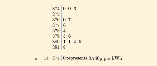
(a) Draw a stemplot of all 14 prices shown in the table.
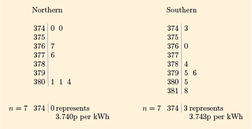
(b) Draw separate stemplots for the seven prices for northern cities and the seven prices for southern cities.
(c) For each of these three batches (northern cities, southern cities and all cities) find the median and the range. Then use these figures to find the general level and the range of gas prices for typical consumers in the country as a whole, and to compare the north and south of the country.
Discussion
For a batch size of 14, the median position is . So, the all-cities median will be halfway between and . These are 3.784 and 3.795, so the median is 3.7895, which is 3.790 when rounded to three decimal places. (The rounded median should be written as 3.790 and not 3.79, to show it is accurate to three decimal places and not just two.)
For the northern and southern batches, both of size 7, the median for each is the value of (that is, ). This is 3.776 for the northern batch and 3.795 for the southern batch.
The range is the difference between the upper extreme, , and the lower extreme, (range ). So the all-cities range is
the range for the northern batch is
and the range for the southern batch is
The medians and ranges are summarised below.
| Batch | Median | Range |
|---|---|---|
All cities |
3.790 |
0.078 |
Northern cities |
3.776 |
0.064 |
Southern cities |
3.795 |
0.075 |
Thus the general level of gas prices in the country as a whole was about 3.790p per kWh. The average price differed by only 0.078p per kWh across the 14 cities.
The difference between the median prices for the northern and southern cities is 0.019p per kWh , with the south having the higher median.
The analysis does not clearly reveal whether the general level of gas prices for typical consumers in 2010 was higher in the south or in the north, though there is an indication that prices were a little higher in the south. The range of prices was also rather greater in the south. It is worth noting that the differences in gas prices between the cities in Table 3 were generally small, when measured in pence per kWh – although, with a typical annual gas usage of 18 000 kWh, the price difference between the most expensive city and the cheapest would amount to an annual difference in bills of about £14 on a typical bill of somewhere around £700.
Activity 2 illustrates two general properties of sub-batches:
The range of the complete batch is greater than or equal to the ranges of all the sub-batches.
The median of the complete batch is greater than or equal to the smallest median of a sub-batch and less than or equal to the largest median of a sub-batch.