3.8 Using a spreadsheet to model project evaluation
In practice the factors to be included in a project evaluation decision are likely to be more detailed and complex than in the examples above. It is useful to model them in a spreadsheet that can be used for different projects and to allow different scenarios to be analysed quickly and easily. In this section we will work through an example of a spreadsheet designed for this purpose.
You will watch four videos which show you how to build a spreadsheet discounted cash flow model. The four videos show a range of techniques and complement each other so watch them in the order they are presented. In your first viewing, watch the four videos one after the other. They are:
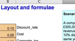
- Layout and formulae
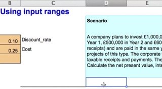
- Using input ranges
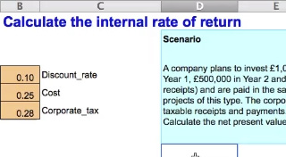
- Calculate the internal rate of return
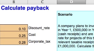
- Calculate payback
All the videos use the following investment scenario:
A company plans to invest £1,000,000 in a new product that will generate revenues (cash receipts) of £300,000 in Year 1, £500,000 in Year 2 and £600,000 in Years 3 to 5. Costs (cash payments) will be 25% of revenues (cash receipts) and are paid in the same year as the relevant cash receipts.
This company uses a 10% discount rate for projects of this type.
The corporate tax rate is 28%. Taxation cash flows occur in the same year as the relevant taxable receipts and payments. There are no taxation cash flows arising from the investment of £1,000,000.
Calculate the NPV, the IRR and the payback period of this investment.
Now watch the videos:

Transcript: Video 1 Layout and formulae
This spreadsheet shows a discounted cash flow or DCF model of the details presented in the investment scenario. Some of the scenario details have already been entered in the spreadsheet, such as the initial investment and the predicted revenues over the five-year period. We have already set an input range. This contains details of items in the scenario that will have a relationship with other items, for example, the corporate tax rate, which is used to calculate the amount of corporate tax payable, 28%.
The time horizon of the investment is five years so the DCF has six columns. Year 0 is the start of Year 1, the point at which the investment is made and the project begins.
Remember the initial investment is a present value. Notice that the initial investment has been entered as a negative cash flow, a negative one million pounds, which is paid out at the start of the project. Revenues are positive cash flows. The project will generate cash receipts of £300,000 in Year 1, £500,000 in Year 2, and £600,000 in Years 3 to 5. Remember we call these future values – amounts received in future time periods.
Now look at the costs, which are negative cash flows. From the scenario, we know that costs will be 25% of revenues and are paid in the same year. The DCF spreadsheet has calculated these costs using a formula. Let’s look at the formula. It’s a minus value. The value of the revenues for Year 1 is taken from cell E14, £300,000, multiplied by the cost. In the input range cost is set at 25% of revenues. So, by using the word ‘Cost’ in the formula, we calculate cost as 25% of revenues.
Next we need to calculate taxable cash flows by subtracting costs from revenues. We call this a memorandum or memo row because it is a note of something we need to calculate. Note that these values are outlined in black and will be excluded from the final net cash flow calculated. Using formula, the spreadsheet calculates a taxable cash flow which, for Year 1, is revenues of £300,000 less costs of £75,000 which gives a taxable cash flow of £225,000. Let’s look at the formula. It is the sum of the cash receipts, a positive number, and cash payments, a negative number.
In the taxation row, taxation is calculated as £63,000. The corporate tax formula entered in this cell calculates the corporate tax percentage of the taxable operating cash flows in that year. Here Year 1 taxable cash flow of £225,000 from cell E16 is multiplied by the corporate tax rate. By using the word ‘Corporate_tax’ in the formula, we can use 28% as the multiplier, as this has been entered in the input range.
The net cash flow calculates a total of the relevant cash flows in the time period. In Year 1 the only relevant cash flow is the investment so this will be minus a million pounds. In subsequent years, net cash flow is the total of the cash receipts, the costs and the taxation amounts. We can copy this formula for Years 2 to 5. Use auto fill by clicking on the bottom right-hand corner of the range to do this.
Now let us enter the discount factor as a formula. The formula is one divided by one plus the discount rate, with the denominator being raised to the power of the time period. In Year 0, the time period is zero, giving a discount factor of one. We can see the effect if we copy the formula into the columns for Years 1 to 5 using auto fill. Discount factor cells have been formatted to show the result to three significant figures.
The next step is to calculate the present value. The DCF spreadsheet has already been set up to calculate present values. We do this by multiplying the net cash flow by the discount factor. To calculate the net present value of this project we sum the present value in Year 0 and the future values in Years 1 to 5.
Note that the net present value is shown to 2 decimal places. In this case the net present value is positive so this project should be undertaken by the company.

Transcript: Video 2 Using input ranges
The investment scenario details have already been modelled in a discounted cash flow or DCF model. You can see the DCF model here. This DCF model calculates a net present value or NPV. You can see that the taxation row has not yet been modelled and we will complete it now as we look at how to use an input range in a DCF model.
Defining and using a range name in a DCF model means that the name can be used in a formula within a cell in the spreadsheet to calculate results. The value in the range name can be changed once and the effect captured in the overall result. Notice how changing Cost from 25% to 26% will change the overall result.
Using an input range saves having to change multiple cell inputs in order to make a change in assumptions when modelling.
We’ve already set up names for two of the inputs. You can see that these names refer to items in the scenario that will have a relationship with another item in the DCF model. For example, the cost percentage is used in the formula in cell E15 to calculate the values in the cost row. The scenario details tell us that these costs are 25% of revenues.
In order to complete the model and use all the scenario details we will now set up a relevant value for corporate tax. Go to the cell B6. Enter 28% corporate tax rate. Type in 0.28. Put the pointer in cell B6. Go to the name box and type in Corporate underscore tax. Press Enter.
In the cell to the right of the input value, type the range name as it is defined and used by the spreadsheet in the cell, that is Corporate underscore tax. Use the underscore key for any names with two or more words. You will use this name in the spreadsheet model.
Go to where you want to calculate taxation, beneath the taxable cash flow of £225,000. Type negative, using the minus sign, E16 multiplied by the words ‘Corporate_tax’. You can see how the net present value changes as it now includes the corporate tax payment as a relevant cash flow.
Copy the formula to the other cells. Use auto fill by clicking on the bottom right-hand corner of the range to do this The NPV is now £36,314.09.
Note how we can change the corporate tax rate in the range name and the net present value will change. We can change the corporate tax rate to 30% and the NPV goes down.

Transcript: Video 3 Calculate the internal rate of return
This spreadsheet shows a discounted cash flow or DCF model for the details presented in the investment scenario.
Details of the relevant cash flows have been entered. You can see the initial investment, the revenues or cash receipts, the costs or cash payments and taxation cash flows
Input range names have been used to help when setting up formulae in cells. You can see that these range names refer to items in the scenario that have a relationship with another item in the DCF model.
We’ve used formulae in the cells to calculate the costs, taxation, net cash flows, discount factors, present values and net present value.
For this investment scenario, we have calculated an NPV of over £36,000.
The next step is to calculate the internal rate of return or IRR of this investment. Have a separate cell in which the IRR percentage can be shown. In this spreadsheet this is D24. Use the IRR function in Excel by typing in equals IRR and picking up the cash flow from Years 0 to 5. The result calculated is 11.28%. Now go to the discount rate cell in the input range and change the value from 10% to 11.28%. It will display as 0.11.
Now see how the NPV has changed from a positive value to a negative one, minus £102.23. This is close enough to zero to show that discounting the future cash flows using the IRR will give a zero NPV.
You can also find an IRR by using the Goal seek command. Change the discount rate back to 10% in the input range. Go to the NPV cell. Now go to the tool bar and click on Tools and Goal seek. In the dialogue box set cell D22 to value 0 by changing cell B4. Press OK. In the next dialogue box just click OK. See how the NPV becomes zero.
Go to cell B4 and look in the formula bar. The discount rate is given to many significant figures, showing that when we use just 11.28% as the discount rate we will end up with a small positive or negative number for the NPV rather than an exact figure of zero for the NPV. The IRR then is the break-even interest rate of the project’s cash flows.
We will now change the discount rate back to 10%. Note that using a 10% discount rate gives a positive NPV, because the IRR, the break-even rate of 11.28%, is higher than 10%.

Transcript: Video 4 Calculate payback
This spreadsheet shows a cash flow model of the investment scenario details. We will now use the scenario in the details of the cash flow model to calculate the payback period of this investment.
Have a row for the cash flows generated from the scenario. Ensure that the cash flows are in the correct time period according to when they are paid or received and remember to show negative or positive values.
In the cash outstanding row use a formula which calculates how much cash is still outstanding at the end of the time period, according to the payback period approach. For example, at the end of Year 1, the debt is the total of the initial investment and the net cash flow in Year 1. In other words the million pounds invested subtract the £162,000 received in the first year.
This means that at the end of Year 1, cash outstanding is a negative £838,000.
You can see that the payback point is some time in Year 4 as the cash flows change from negative to positive between Year 3 and Year 4.
To find the payback point in years, use the formula in D22 and copy it into other columns for Years 1 to 5. Use auto fill by clicking on the bottom right-hand corner of the range to do this.
This formula uses the IF command to check whether the cash outstanding at the end of each year- is negative or positive. When the cash outstanding at the end of one year is negative but at the end of the subsequent year is positive, the payback period will be calculated. The payback period is 3.75 years.
To see the exact payback point in years and months, copy the formulae from cells D23 and D24 to the end of the project’s time horizon.
Use auto fill by clicking on the bottom right-hand corner of the range to do this.
These formulae convert the payback period in years into years and months. This is a nice feature but not strictly necessary. We could work out the number of months manually. It’s three-quarters of a year or 9 months.
So we can see that for this investment, the payback period is 3 years and 9 months.
You can see the DCF spreadsheet (solution) [Tip: hold Ctrl and click a link to open it in a new tab. (Hide tip)] here.
Spreadsheets can be useful tools for decision making, but it is very important that they are constructed and tested carefully. Research suggests that poorly designed and controlled spreadsheets are reasonably common in business and can cause sizable losses (Powell et al, 2009).
This section has looked at the principles which are the foundation of the project evaluation. These include what information to include in an appraisal, using concepts such as relevant cash flows, sunk costs and opportunity costs. The time value of money and how project appraisals account for it by using a discount rate were discussed. Some approaches to estimating the discount rate, and their advantages and disadvantages, were discussed and the use of a spreadsheet to model discounted cash flow decisions introduced.
When performing project appraisal for decisions in practice, you would need to decide what the appropriate discount rate to use is, and the information in this section should help you do that. The guidance about designing a spreadsheet should also assist in applying this understanding to practical situations, but note the warning from research studies that it is important to be very careful using any tool - but spreadsheets in particular!
