Estimating the cost of equity
Use 'Print preview' to check the number of pages and printer settings.
Print functionality varies between browsers.
Printable page generated Friday, 29 May 2026, 5:25 PM
Estimating the cost of equity
Introduction
In this free course we examine the factors that determine the return sought by investors when buying shares. This expected return takes into account the perceived risks of investing in different shares.
Section 1 of this course should be used in conjunction with the activities provided in Sections 2 to 5. The latter will help you develop and test your understanding of the concepts and issues covered.
This OpenLearn course is an adapted extract from the Open University course B858 Introduction to corporate finance.
Learning outcomes
After studying this course, you should be able to:
select and justify a suitable risk-free rate and equity risk premium for use in determining the expected return for a share
evaluate the different approaches to identifying a suitable equity risk premium
use the dividend valuation model to calculate the return on a share and the return on a market
use the return on a market to arrive at an implied equity risk premium.
1 Estimating risk and return for shares
Commercial organisations discount projected cash flow by an appropriate discount rate to determine whether they offer an adequate return on the necessary investment. Financial investors look to those same commercial organisations to provide a return on their money. This section examines the importance of determining, or more often estimating, the required return on an investment.
1.1 Rewarding risk
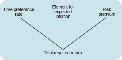
The return required by investors for making any form of investment is based on three key determinants:
- A time preference rate. This is the return required to persuade investors to give up the ability to use their cash for consumption today in favour of investing the cash to provide a return over a future time period.
- An element for expected inflation. This is required to ensure that the purchasing value of the money invested keeps pace with the expected rate of price inflation. Without this investors could find that the value of their investment after accounting for the impact of inflation is worth less than at the inception of the investment.
- A risk premium. This is required to reward investors for the risk that they may not receive back all or any of the money they invested – for example, if the company invested in becomes bankrupt and defaults on its financial obligations.
These factors that underpin the expected return on an investment are set out in Figure 1
When it comes to investments in shares we need to develop these three elements that determine the expected return to investors.a
For shares the return is subdivided into three different elements:
- a risk-free rate
- an equity risk premium
- a reward adjustment for the volatility of the share relative to the share market as a whole.
This is shown in Figure 2.
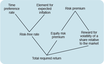
The risk-free rate in Figure 2 includes two of the three elements set out in Figure 1: a time preference rate and a reward for expected inflation. The risk premium from Figure 1 is now subdivided into two elements: a risk premium for shares (or equities) generally and a reward adjustment for the relative volatility of a particular share compared with the share (or equity) market as a whole. Both Figures 1 and 2 show different constituent elements of the required return on equity by investors.
In this course we will look at the first two elements of the required rate of return on a share as shown in Figure 2: the risk-free rate and the equity risk premium.
The third element – the reward adjustment for the volatility of a share relative to the market – is an adjustment that investors make to accommodate the perceived riskiness in investing in the shares of a specific company relative to the average risk of investing in the equity market.
1.2 The risk-free rate
Investors expect to be rewarded for taking on extra risk. However, even if an investment is free of risk, investors still require a reward. This is to compensate for time preference and to include an element for expected inflation. The ‘real’ rate of return is the rate of return investors require after allowance has been made for expected inflation.
The nearest thing to a completely risk-free investment is a government security, such as a short-term Treasury bill (with a maturity of up to one year) or longer-term government bonds. Lending to a government is generally (but not universally) free of the risk that the investor will not receive either the interest or the capital when the loan comes to be repaid. This reflects the fact that most governments do not need to default on their domestic debt (i.e. debt denominated in the currency of that country) – they can just create more money to repay investors (this is obviously not true for the countries that have joined the eurozone). For heavily indebted governments, too much money creation may cause high inflation, and therefore reduce the real value of the bond repayments. So, although the debt may be repaid in full, there is no guarantee that the real rate of return will be as high as was initially expected.
Stop and reflect
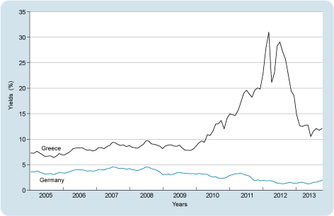
Look at Figure 3 that shows Greece’s borrowing costs relative to Germany’s during the period 2005–13. Why did the cost of Greek debt become much higher than the cost of German debt?
Greece is a member of the eurozone. Before it joined, it issued bonds in its own currency, the Greek drachma, and repaid as it wished using its own currency. In 2010, Greek government debt was denominated in euros but the Greek government did not have control over this currency. No individual government in the eurozone has the right to issue unlimited amounts of euros – the currency is ‘owned’ by the participating states as a group.
Figure 3 shows the returns (yields) required by investors for lending for ten years to the Greek or German governments (2005–13). Up to mid-2008, there was barely any difference between the two government yields. From 2008 onwards, the perceived risk of Greek government bonds was higher than for German government bonds and investors began to require higher yields on Greek bonds. By early 2010, there was a real risk that Greece would have to default on its debt, as the economic recession had reduced the Greek government’s income. Investors raised the amount they required to lend to the Greek government dramatically to well above the amount required to lend to the German government (even though Germany also uses the euro and is part of the eurozone). In May 2010, the International Monetary Fund (IMF)* and the eurozone countries agreed a €110bn loan to Greece. This did not have any significant dampening effect on long-term Greek government bond yields. These yields kept on rising until February 2012 when a debt ‘haircut’ deal - a writing down of the face-value of Greek bonds - of €206bn, accompanied by a second bailout package (a new €100 billion loan and a retroactive lowering of the bailout interest rates), was agreed. Investors were asked to write off 53.5% of the face value of the Greek sovereign bonds they were holding.
* The International Monetary Fund (IMF) describes itself as an organisation of 187 countries, working to foster global monetary cooperation, secure financial stability, facilitate international trade, promote high employment and sustainable economic growth, and reduce poverty around the world. For more information, go to www.imf.org/ external/ about.htm.
Treasury bills can be considered to be the safest investments available on the international capital markets, given the credit-worthiness of (most) governments, their short-term nature and the fact that they can be easily bought and sold. As you saw in earlier, the returns offered on investments include an element for expected inflation. If inflation turns out to be lower or higher than expected, investors will earn more or less in real terms than they expected. This is known as inflation risk. The short maturity of Treasury bills, however – one, three, six or even 12 months – minimises the likely difference between actual and expected inflation and hence their inflation risk is almost nil.
Treasury bills in most countries are traded in large nominal amounts. In the UK, the minimum nominal amount is £500,000.
The return offered on Treasury bills can be considered to be almost a risk-free rate and the minimum required rate of return for all investors. All other securities are considered to be riskier than Treasury bills, in the sense that they are more volatile in their price movements (i.e. they have a higher standard deviation of returns) or they carry a greater risk that the borrower will not repay the debt. These securities should offer investors an expected rate of return at least as high as the return offered on Treasury bills.
An alternative estimate of the risk-free rate of return is obtainable on long-term government bonds. This definition is often preferred by managers when determining a benchmark risk-free rate because, they argue, they are typically looking at long-term projects and their investors are looking to invest over the long term. Over longer periods, an investor’s risk-free alternative would be to invest in a government bond of the same maturity as their desired holding period and earn a promised yield to maturity. Figure 4 explains how to understand UK government bond terminology, such as the interest paid on the bond (known as the coupon), its title and its maturity or redemption date.
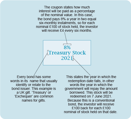
UK government bonds are called gilts – the certificates used to be gilt-edged and as the UK government has never defaulted on a debt, they can be considered as secure as gold!
Treasury bills and long-term government bonds can be considered essentially risk free. Note, however, that the return expected from a Treasury bill is likely to differ from the return expected on, say, a 20-year government bond, since investors require different returns on investments with different maturities. These different returns are often described as the term structure of interest rates and can be shown graphically in what is called a yield curve, where the yield on the y-axis (or vertical) is plotted against maturity on the x-axis (or horizontal).
Remember that all yields or interest rates are given on an annualised basis for ease of comparison. In the text, p.a. stands for per annum.
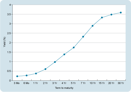
Figure 5 shows the yield curve for UK government bonds, or gilts starting at three months and stretching out to 30 years at a particular point in time (in this case, 16 December 2013). So, on that day, investors required only just over 20 basis points (or just over 0.20% since there are 100 basis points in one percentage point) for lending for three months to the UK government. In contrast, investors required 2.89% p.a. for lending for 10 years, 3.48% p.a. for lending for 20 years and 3.59% p.a. for lending for 30 years. This means that, the longer the maturity of the bond (i.e. the further away its redemption date), the higher the annual rate of return or yield to maturity that they require. This is called a rising yield curve.
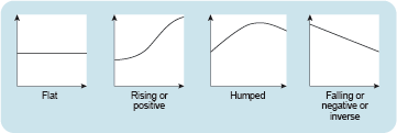
Yield curves can be flat, rising, humped or falling depending on investors’ expectations about the future levels of interest rates. Figure 6 shows the alternative yield curves. The simplest way to explain why there are different shapes of yield curve is to do with expectations, the so-called expectations hypothesis. For example, if investors expect rates to go up in the future, the yield curve will be rising; if investors think they will go down, the yield curve will slope downwards. Flat yield curves are due to an expectation that interest rates will remain unchanged. However, supply and demand also influence yield curves. For example, if there is demand from banks for short-term government bonds and demand from long-term investors such as pension funds for long-term government bonds, there may be a lack of demand for bonds of medium maturity – say five to ten years. In such a case, the yield curve might well be humped, with the highest yields available on medium maturity bonds.
Stop and reflect
What do you think the yield curve would look like for a country with financial problems and a higher risk of default than the UK (for example, Greece before the rescue package in May 2010)?
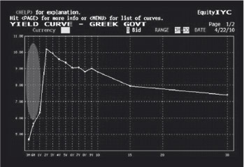
The shape of the curve depends on when you take your snapshot. Figure 7 shows the yield curve for Greece on 22 April 2010 just before the rescue package was announced in early May. In such a severe crisis situation, the curve was falling; one to three-year bonds had a much higher yield than, say, 30-year bonds. Greece was either expected to default in the short term or survive and improve.
We will now examine the second element of the required rate of return on a single share: the equity risk premium.
1.3 The equity risk premium
For details of companies listed on the London Stock Exchange, go to www.londonstockexchange.com/ statistics/ home/ statistics.htm. For details on the different FTSE indices, go to www.jrank.org/ finance/ pages/ 2031/ FTSE-Indexes.html.
The overall or average rate of return on shares or equities can be measured by the rate of return on a stock market index. This is a number designed to reflect the returns (dividends plus capital gains or losses) of shares that are representative of the stock market as a whole. It is the rate of return you would obtain if you invested in every company share traded in the market, weighted for each company’s relative size. In practice, there are a number of stock market indices available for each stock market. Some indices are designed to reflect only the performance of the largest companies, but an index designed to reflect the market as a whole is needed here. In the UK, this is the FTSE-All Share Index that actually only covers around 700 shares out of the 2,700 or so listed, but these shares account for 98% of total market value and 90% of turnover by value.
Equities on average have higher returns than bonds because of their greater risk, with risk usually measured by the standard deviation of the returns. This has been demonstrated by Dimson et al. (2002) using historical returns during the period 1900–2000. They showed that, during this period, UK equities achieved mean annual nominal returns of 12.1% compared with 6.1% for UK gilts. Their work also demonstrated how three-month UK Treasury bills yielded, on average, an annual 5.1% in nominal terms over the same period. Therefore, in the past, companies raising equity finance have offered higher returns to their shareholders than what was available on risk-free assets in order to compensate for the additional risk of equities.
This difference between the return on equity measured by the return on a stock market index and the risk-free rate is known as the equity risk premium or market premium (The term ‘equity risk premium’ is used here but you may see the term ‘market premium’ elsewhere). This premium is usually calculated as the simple difference between the two. Based on the historical data on nominal returns for the period 1900–2000 (Dimson et al., 2002) and using Treasury bills as the risk-free investment, the equity risk premium was 12.1% – 5.1% = 7%. If, instead, long-term government bonds were used as the risk-free benchmark, the market premium was somewhat lower: 12.1% – 6.1% = 6%. This implies that, on average, over the last 100 years or so, equity investors have earned between 6% and 7% each year as a premium for taking on the risk of buying shares rather than investing in risk-free government bonds. Note the use of the phrase ‘on average’: in any one year or decade, returns could be much higher or lower than expected and certainly might differ substantially from the long-run average market premium achieved in the 20th century.
Stop and reflect
Can an equity risk premium be negative?
For the decade from 2000 to 2009 inclusive, including the credit crunch [2008–9 global financial crisis], the realised equity risk premium was a depressing –2.5% compared with Treasury bills and, even worse, –3.1% compared to government bonds. This shows the difference between the actual and expected equity risk premium. Investors putting their money into the stock market in January 2000 cannot have expected a negative equity risk premium, but that is what they got! Luckily, events such as the credit crunch do not happen very often.(Source: Credit Suisse Research Institute, 2010, p. 47)
1.3.1 Estimating the future equity risk premium
There are three ways to estimate the future equity risk premium:
- using historical data and assuming that the past equity risk premium is a good indicator of the future equity risk premium
- asking experts for their opinion of the future equity risk premium
- estimating the implied future equity risk premium from today’s stock market index value using the dividend valuation model (DVM).
Using historical data
This method takes into account past returns on equities and risk-free assets and looks at the actual difference. It assumes that the average equity risk premium that was earned in the past is the same as investors expect to earn in the future. There is an assumption that the actual equity risk premium earned reflects what investors expected the equity risk premium to be before investing. In other words, the extra 6% or 7% that investors earned in the past by investing in equities rather than risk-free assets is assumed to be a reliable indicator of what investors expect today for the future.
When looking at the past, it is essential to get enough data points for statistical reliability. For example, taking ten years of annual data would not give a reliable estimate of the future equity risk premium, as we have seen already. A 100-year period, that Dimson et al. (2002) use, gives a much more reliable estimate of the average historic equity risk premium from which to derive an expected future equity risk premium.
Stop and reflect
Why is the historical equity risk premium approach not appropriate for estimating the equity risk premium for markets such as India or China?
It is not appropriate because there is not enough reliable historical data for such markets.
One advantage of looking at the historic equity risk premium and not just historic equity returns, is that, by doing so, the effects of inflation are neutralised. Both historic bond yields and historic equity returns will have included an allowance for inflation and so, by taking the difference between these two numbers, the equity risk premium becomes inflation neutral. Including data from the 1970s, for example, when inflation was very high, should not distort the results.
Expert opinion
Another way of estimating the expected future risk premium is to ask the experts. For example, what do fund managers or academics think that the equity risk premium should be in order to compensate investors for the extra risk of investing in equities when compared with the risk-free asset? Such experts should know about the historic returns for estimating the future equity risk premium, but they may also have additional insights as to possible special factors to allow for in the future (e.g. the impact of the 2008–9 global financial crisis).
In 2010, a global survey of 3,861 analysts, company managers and university professors gave the replies shown in Table 1 when they were asked for the equity risk premium relative to bonds that they used in their calculations of present value of future cash flow. Note that their equity risk premium expectations are below estimates derived from long-run historical data. For example, the UK equity risk premium forecasts in Table 1 are between 5.0% and 5.6% which is less than the 6% historic equity risk premium for the UK (calculated on 100 years of historical data).
| Group | Average ERP | |||
| USA and Canada | Europe | UK | Other (emerging markets) | |
| 601 analysts | 5.1% | 5.0% | 5.2% | 6.3% |
| 1,749 corporate managers | 5.3% | 5.7% | 5.6% | 7.5% |
| 1,511 professors | 6.0% | 5.3% | 5.0% | 7.8% |
Stop and reflect
Why do you think there is much similarity in the estimates for developed markets? Why do you think the estimate is higher for other (emerging market) countries?
The lack of difference in the equity risk premium estimates for the major stock markets is probably due to the globalisation of US finance texts and hence of views on the equity risk premium.
The higher equity risk premium applied by emerging market country managers and analysts may be due to the less developed corporate governance, stock market regulation, accounting disclosure and legal protection for minority investors in those markets.
The dividend valuation model
The third method of calculating the equity risk premium is to estimate the implied equity rate of return embedded in the current market price, given the forecast dividends to be paid on shares. To do this, the dividend valuation model is used. Dividends are the payments made to share investors by companies – usually once or twice a year.
The dividend valuation model (DVM) simply defines the price Pi of a share i to be the present value of all future dividends discounted by the required rate of return for that particular share. Since companies have an unlimited life, provided they are not liquidated, an infinite stream of dividends, Dn, from year 1 to infinity, ∞, can be assumed. So:
- where
- Pi = current price of share i
- Dn = dividend expected in year n on share i
- E(Ri) = expected return on share i given its risk
- (∑ means the summation of all terms with n varying from n = 1 to n = ∞ (infinity).)
This is a simple present value equation that does not depend on any unrealistic assumptions to be valid. Its disadvantage, however, is that no one really has any idea what the likely dividends are going to be for any company, given the uncertainties of the real world.
A simplified version of the DVM, sometimes known as the Gordon growth model after Gordon (1959), assumes for simplicity that dividends will grow at a constant rate, g. Although unrealistic, the advantage of the Gordon growth model is that the formula simplifies dramatically to:
- where
- Pi = current price of share i
- D1 = dividend expected in year 1 on share i
- E(Ri) = expected return on share i given its risk
- g = expected constant annual growth rate of share i’s dividends
- Multiplying through by E(Ri) – g, dividing by Pi, and taking g to the right-hand side of the equation gives:
This can be interpreted as saying that the required rate of return on a share is the sum of the dividend yield (with next year’s dividend rather than last year’s) and the expected growth rate, g, on the dividends. Therefore, the cost of equity capital for a share or market can be estimated by inputting the expected dividend for next year and dividing by the current share price (or, taking the expected dividend yield), and then adding the expected constant growth rate for dividends beyond next year. This growth rate can either be estimated by assuming that the historic growth rate over, say, the last five years will continue indefinitely, or can be derived from consideration of a likely real rate of growth (which could be assumed to be the long-term real growth rate of the economy) plus a long-term forecast inflation rate.
Note that the Gordon growth model formula (1959) was obtained by using the idea of a geometric progression; that is, a progression where each term grows by a constant factor. In the case of the Gordon growth model, the factor includes (1 + g) which is what the dividends grow by each year.
Example
A share has an expected dividend next year of 3p, a current share price of 100p and its historic growth rate in dividends has been 8% per year.
The cost of equity capital can be estimated as:
E(Ri) = D1/Pi + g = (3/100) + 8% = 3% + 8% = 11%
if it is assumed that dividend growth in the future will be the same as in the past.
Alternatively, suppose the long-term inflation forecast is 5% annually and the company is expected to grow in line with the economy, which is expected to grow 2.5% in real terms every year. The Fisher equation provides a formula for the relationship between nominal and real growth for interest rates, which can be applied to the nominal growth rate as:
1 + nominal growth rate = (1 + real growth rate)(1 + expected inflation)
So,
Substituting into the Gordon growth model, the cost of equity capital for this company can be estimated as:
E(Ri) = D1/Pi + g
= 3% + 7.625% = 10.6%, rounded to one decimal place.
Note that many investors approximate the above version of the Fisher equation by simply adding the real growth and expected inflation components. In this case, it would be 2.5% + 5% = 7.5% rather than 7.625% for g.
This formula can also be applied to the market as a whole to estimate the equity risk premium implied by current market prices and dividend forecasts. In December 2010, the UK market, as measured by the FTSE All-Share Index, had an overall dividend yield of 3% and, by consensus, the expected growth rate of UK dividends for that index was 7.5% (equivalent to approximately 2.5% real growth in dividends and 5% expected inflation). If the government bond yield at the time was 4.0%, what was the expected equity risk premium?
Using the formula E(RM) = D1/PM + gM where D1/PM is next year’s dividend yield for the market as a whole and gM is the growth rate expectation for the market as a whole, gives D1/PM = 3% x (1.075) = 3.225% and gM = 7.5% and so E(RM) = 10.725%. Deducting 4.0% for the risk-free rate gives an equity risk premium implied by the market of 6.725%, above the historic estimate of 6% (assuming a bond benchmark) and the expert forecasts of 5.0% to 5.6%.
2 Worked examples – Estimating risk and return for shares
View the animations on the following pages to see worked examples using formulae from Section 1: Estimating risk and return for shares.
You can use the animations in a variety of ways:
- Play and watch the animation from beginning to end.
- Review the calculation task and pause the animation while you find the solution on your own. Continue playing the animation to check your own solution.
- To revise, check your own worked solution against that shown in the animation.
You can play the animations as many times as you want.
Dividend valuation model (DVM)
Throughout this course, we use the Gordon Growth variation of the dividend valuation model (DVM). The Gordon Growth model assumes constant growth in dividends.
Play the animations below to see worked examples of the mathematical techniques covered in this course.
These examples show you how to:
- use the DVM to calculate the expected return on a share
- use the DVM to calculate the expected return on a share using the share’s dividend yield
- find the equity risk premium (ERP) using:
- a dividend yield
- growth expectations for dividend yield and
- the risk-free rate. This is the third way of estimating an ERP.
These examples use the dividend valuation model (DVM), which is explained in the text you read at the start of the course.
2.1 Calculate the expected return on a share I
View the video to see the first in a series of three worked examples showing how to calculate the expected return on a share.
Transcript: Calculating expected return part 1
Calculate the following:
(a) the expected return on a share where:
the expected dividend next year is 10 pence,
the current market value of the share is 90 pence, and
the growth rate in dividends is forecast at 6 per cent
(b) the dividend yield using next year’s expected dividend.
Part (a). Let’s use the Gordon Growth variation of the dividend valuation model, which is rearranged to find the expected return, whereby the expected return on a share (E(Ri)) is equal to the expected dividend next year (D1), divided by the current price of the share (Pi) plus the growth rate of dividends (g) from investing in the share.
Let’s put the figures from the question in: 10 pence divided by 90 pence, plus the growth rate of 0.06 or 6 per cent.
Therefore, the expected return on the share is 0.1711 or 17.11 per cent.
Part (b).To find the dividend yield, we can divide the expected dividend next year (D1) by the current price of the share (Pi).
This means that we divide 10 pence by 90 pence. It gives us a dividend yield of 0.1111 or 11.11 per cent.
2.2 Calculate the expected return on a share II
View the video to see the second in a series of three worked examples showing how to calculate the expected return on a share.
Transcript: Calculating expected return part 2
The growth rate of dividends in B plc is expected to keep pace with a future long-term inflation rate of 3.5 per cent and the historic real rate of growth of B plc, which has been 2 per cent.
B plc has just paid the current year’s total dividend of 1 euro and 40 cents and the current share price is 16.00 euros. Calculate the expected return for B plc’s shareholders.
To find the nominal growth rate, we will use the Fisher equation, where 1 plus the real rate, multiplied by 1 plus the expected inflation rate, equals 1 plus the nominal rate.
Let’s put the figures from the question in: 1.02 multiplied by 1.035 equals 1 plus the nominal rate.
Let’s now find the nominal rate: 1.0557 subtract 1 equals 0.0557. Therefore, the nominal growth rate is 5.57 per cent.
Let’s use the Gordon Growth variation of the dividend valuation model which is rearranged to find the expected return, whereby the expected return on a share (E(Ri)) is equal to the expected dividend next year (D1), divided by the current price of the share (Pi) plus the growth rate of dividends (g) from investing in the share.
To find the dividend next year we multiply 140 cents (if we work in cents) by 1.0557, divide this by 1,600 cents and then add the growth rate of 0.0557 or 5.57 per cent.
Work out the fractional term, which gives us 0.0924, and then add the growth rate of 5.57 per cent. This gives us an expected return for B plc’s shareholders of 0.1481 or 14.81 per cent.
2.3 Calculate the expected return on a share III
View the video to see the third in a series of three worked examples showing how to calculate the expected return on a share.
Transcript: Calculating expected return part 3
D plc has a dividend yield, based on this year’s total dividend, of 5 per cent. Given that the forecast growth rate of the dividend yield for D plc is 3 per cent, what is the expected return for a shareholder?
Let’s use the Gordon Growth variation of the dividend valuation model which is rearranged to find the expected return, whereby the expected return on a share (E(Ri)) is equal to the expected dividend next year (D1), divided by the current price of the share (Pi) plus the growth rate of dividends (g) from investing in the share.
D1 divided by Pi is the dividend yield of 5 per cent
So take 0.05 or 5 per cent which is the dividend yield and multiply by 1 plus the growth rate, 3 per cent. This will give the dividend yield for next year.
Then we need to add the growth rate of 0.03 to the dividend yield for next year.
Therefore, the expected return for a shareholder in D plc is 0.0815 or 8.15 per cent.
2.4 Find the equity risk premium (DVM approach)
View the video to see a worked example showing how to find the equity risk premium using the DVM approach.
Transcript
Find the US equity risk premium if this year’s dividend yield for the US stock market is 5 per cent, the expected growth rate of US dividends in the US stock market is 6 per cent, and the US risk-free rate is 4.5 per cent.
Let’s use the Gordon Growth variation of the dividend valuation model which is rearranged to find the expected return, whereby the expected return on a share (E(Ri)) is equal to the expected dividend next year (D1), divided by the current price of the share (Pi) plus the growth rate of dividends (g) from investing in the share.
Use this formula to find the return on the US stock market using the market data given.
Use the dividend yield for the US stock market, which is 5 per cent. It is expected to grow at 6 per cent. So we need to multiply 0.05 by 1.06 and then add the growth rate of 0.06 in order to work out the expected return on the US stock market.
This becomes 0.053 plus 0.06, which gives us 0.113 or 11.3 per cent.
We can now find the equity risk premium. Take the expected return on the market (E(RM)) subtract the risk-free rate (RF) to find the equity risk premium.
The expected return on the market is 11.3 per cent. Subtract the risk-free rate of 4.5 per cent. This gives an expected risk premium of 6.8 per cent.
3 Practice activities – equity risk premium (ERP)
The following pages contain a range of activities to help you get to grip with equity risk premiums.
Find a risk-free rate
In Activity 1: Finding a risk-free rate, you will see how to find a risk-free rate for use at home (local projects in a local or home currency) and abroad (projects in a foreign location in a foreign currency).
In Activity 4: Finding an equity risk premium, you use Bloomberg to explore the ERP in different locations (the US, China and Indonesia).
Bloomberg is the name given to a software system that provides financial news and information, both historic and real-time. It also provides the basis for a trading system for financial transactions, such as buying and selling bonds.
Bloomberg estimates an ERP using financial data from stock markets. That is, finding an implied ERP from the stock market yield, the consensus view of growth rates and the risk-free rate. Evaluate the Bloomberg approach in Taking on the market.
Key people in corporate finance
 | The equity risk premium Aswath Damodaran is a Professor of Finance at the Stern School of Business at New York University and has produced a number of finance texts. He also maintains a website with a wealth of financial spreadsheets and seminar presentations on corporate finance techniques, particularly valuation topics. Damodaran’s website provides his views on the current risk-free rate and equity risk premium, which he regularly updates. He calls himself first and foremost a teacher and advocates a ‘dose of common sense’ when working with corporate finance techniques and concepts. If you have time and are interested, visit Damodaran's website and/or carry out a wider internet search. |
3.1 Finding a risk-free rate
Complete the activity below to find a risk-free rate.
Activity 1 Finding a risk-free rate
Recommend a suitable risk-free rate to a UK analyst for use in arriving at an appropriate discount rate to discount a fourteen-year cash flow.
Hint: look at the UK–GILTS cash market table from the Financial Times which reports prices. Choose a suitable redemption yield (‘Red Yield’) for discounting a ten-year cash flow. This table has market prices from 20 November 2013.
Add your notes here.
Feedback
Use the fourteen-year gilt yield, which is 3.12%. Look for the ‘Red Yield’ or redemption yield, against the Treasury 4.25% 2027 or ‘Tr 4.25pc ‘27’.
We suggest the yield on the 2027 gilt because it shows expectations of the risk-free rate over the next 14 years (from 2013) and we want to evaluate a 14-year cash flow.
The ‘short’ gilt, such as the Treasury 5% 2014, would not be appropriate.
The redemption yield is the yield of the bond when held to maturity or redemption and takes into account the price paid.
The latter offers a redemption yield of 0.81%, showing how the view of UK interest rate expectations is reflected in the yields of gilts (UK government-issued bonds). In January 2011, interest rates were expected to increase over a period of time to 2021.
Point to note…
Consider the time period of investment when identifying a suitable risk-free rate.
Also, consider macroeconomic factors. On 20 May 2013, the redemption yield on the 14-year gilt (Treasury 4.25% 2027) was 2.51%. Why?
The lower price was a response to the macroeconomic events in May 2013 and the volatility (creating uncertainty for investors) in financial markets, particularly equity markets. The demand for gilts pushed the price of gilts up and the result was falling yields.
Finding a risk-free rate
You can find this information online. By going to the FT markets data web page, you can access a range of archived financial markets data.
Within the data archive section, you can set the category to ‘Bonds & Rates’, set the report to ‘UK Gilts – Cash Market’, and set the date that you want.
3.2 Choosing a risk-free rate
Complete the activity below to choose a risk-free rate.
Activity 2 Choose a risk-free rate
Question 1
A US analyst is selecting a risk-free rate in order to evaluate a 15-year project located in Brazil. The project’s cash flows are in Brazilian reals.
1. Which risk-free rate would be appropriate: US or Brazilian?
Feedback
The most appropriate risk-free rate is one that reflects the risk of the location (of the project or investment).
Remember that the risk-free rate comprises the time preference rate and the inflation rate. The Brazilian and US economies will have different expectations of inflation and this will be reflected in their risk-free rates. The cash flows from an investment located in Brazil will be influenced by inflation in Brazil. So, use a Brazilian risk-free rate.
Question 2
2. What if the project’s cash flow is in dollars, but the risk of the location stays the same?
Feedback
An alternative approach would be to use a 15-year US Treasury bond yield plus a country risk premium for Brazil.
This approach can be used with Brazilian currency cash flows by converting the project’s cash flows from Brazilian reals to US dollars.
Doing this overcomes the difficulty of obtaining a risk-free rate for a project based in a location where the government does not issue government-backed bonds that would provide a risk-free rate.
Point to note...
Consider the location of the investment.
3.3 Calculating a risk-free rate
Complete the activity below to calculate a risk-free rate.
Activity 3 Calculating a risk-free rate
Question 1
You are considering investing in an Indian company, in rupees.
Calculate a risk-free rate using:
- a.Bloomberg, which gives you the following figures for India:
- Return on the market = 13%
- Equity risk premium = 5%
- b.information given by a US bond rating agency about an Indian government bond, as follows.
The Indian government has a rupee-denominated bond that currently yields 14%. The US bond-rating agency (Standard and Poor’s) has given this bond a rating of A. The current spread over a risk-free rate, for an A-rated country, is 6%.
1. Estimate the rupee risk-free rate.
Hint: to arrive at a suitable risk-free rate, deduct the bond risk premium (6%) from the bond yield.
Add your notes here.
Feedback
Using Bloomberg
The risk-free rate = 0.13 – 0.05 = 0.08 or 8%.
Using the Indian bond market and US rating agency
The risk-free rate = 0.14 – 0.06 = 0.08 or 8%.
According to Standard and Poor’s, Indian government bonds have a risk premium of 6% above the risk-free rate.
Question 2
Government bonds are rated in the same ways as corporate bonds. In 2010, Greek ratings had a rating of BB+ compared to AAA for a US bond. Can you think why the ratings are different?
Add your notes here
Feedback
In 2010, Greece had a higher default risk than the United States.
Standard & Poor’s website provides more information on credit rating and definitions.
Point to note…
Credit ratings are indicative of default probabilities. So, a corporate bond rated ‘AA’ is viewed by Standard & Poor’s as having a higher credit quality and less likelihood of default than a corporate bond with a ‘BBB’ rating. See Standard & Poor’s website for rating definitions.
3.4 Finding an equity risk premium
Complete the activity below to find an equity risk premium.
Activity 4 Finding an equity risk premium
‘Finance is an art. And it represents the operations of the subtlest of the intellectuals and of the egoists.’
The following data was taken from Bloomberg on 13 December 2013. We have extracted three countries for you to review.
The implied equity risk premium is the difference between the market return and risk-free rate. The market return has been calculated using the growth rate. Bloomberg does not give the exact method for its approach but we will accept the results in the table as they are.
| Country | Growth rate (%) (consensus five-year projected growth) | Risk-free rate (%) (yield on ten-year treasury security) | Market return (%) (average yield taking account of all major index companies) | Implied equity risk premium (%) |
| US | 11.85 | 2.87 | 9.98 | 7.12 |
| China | 13.62 | 4.61 | 14.14 | 9.53 |
| Indonesia | 8.80 | 8.56 | 10.13 | 1.58 |
Look at the equity risk premium:
- What reasons can you give for the different premiums?
- What do the differences tell you about the perceived risk and return from investing in companies in those countries?
Hint: information on stock market movement and other economic indicators is available from the Trading Economics website. (Trading Economics (2011) Stock Market Indexes, taken from http://www.tradingeconomics.com. With kind permission.)
Remember that this website will have current information and the Bloomberg equity risk premium ‘snapshot’ given in this exercise was taken in December 2013. If you see any anomalies, think about economic events, both global and country-specific, which may have occurred since December 2013.
Add your notes here
Feedback
There is a huge 7.95% spread between the three equity risk premiums quoted in Bloomberg on 13 December 2013.
We suggest the following:
China offers the highest market return and the highest equity risk premium, reflecting the forecast of China’s future real growth in relation to the risk-free rate.
Indonesia offers the second higher market return, but very close to the relevant US one. The global recession in 2008 took the stock market down to its 2006 level, but the stock market has fully recovered its upward path since then, being stabilised in considerably high levels. Although Indonesia offers the lowest equity risk premium, this is partly due to the very high prevailing interest rates.
A base rate is an interest rate set by banks. This determines borrowing and lending rates.
The US market return is the lowest of the three countries and its historic trend has been affected by the low growth in the wake of the 2008 financial meltdown. At the time of writing, IMF economic forecasts suggest an economic recovery in the future and this anticipation is reflected in the considerably high consensus dividend growth forecast (11.85%). The US equity risk premium is much higher than Indonesia’s due to the low US risk-free rate, which reflects to some extent the low base rate of the Federal Reserve in an effort to kick-start the US economy.
Using an implied approach to calculate the equity risk premium, as in the Bloomberg ‘snapshot’, means that you inevitably take account of historic events captured in the current risk-free rate (such as the lowering of the risk-free rate in the USA). Such events may not happen again in the future.
Point to note…
If you use an implied equity risk premium approach when finding a discount rate for use in a valuation or investment appraisal, consider other factors that contribute to the premium result.
In particular, think of the approach in calculating the market return. The Bloomberg approach is to use the consensus five-year projected growth forecast to calculate the return.
Can you think of any disadvantages of this?
One disadvantage is that you are using a consensus view of future growth that may not materialise.
4 Evaluate – The ways of calculating ERP
While reading 'Estimating risk and return for an individual share', you found three ways to calculate the equity risk premium (ERP):
- using historical data and assuming that the past equity risk premium is a good indicator of the future ERP
- asking experts for their opinion of the future ERP
- estimating the implied future ERP from today’s stock market index value (using the dividend valuation model).
In the following three activities you will:
- identify and evaluate the ERP put forward by Professor Aswath Damodaran
- read ‘The new premium puzzle’, which highlights the challenges of arriving at an ERP
At the end of these activities, make notes on the advantages and disadvantages of the three methods used to arrive at an appropriate ERP.
4.1 Identifying the ERP
Complete the activity below to identify the ERP.
Activity 5 Identifying the ERP
Question 1
1. Identify and evaluate the approach of leading US academic analyst, Professor Aswath Damodaran:
Prior to September 2008, I used 4% as the ERP based on an estimate of the average implied ERP over the period 1960–2007. The banking and financial crisis of 2008 was unlike any other market downturn and exposed weaknesses in developed capital markets. After the crisis, in the first half of 2009, I used an ERP of 5.5% when valuing companies. However, in the later part of 2009, I saw a reversion to historical averages and an ERP of 4.5–5% now seems appropriate for 2010.
Feedback
Professor Damodaran uses an implied ERP calculation, based on past evidence (historical averages). This has then been adjusted to take account of the extreme events of 2008 using personal bias.
The expert’s decision to adjust the ERP upwards reflects a view that it will be more difficult to achieve the required gains from stock market investments and thus investing in stock markets carries increased risk.
In 2008, global share prices decreased sharply as investors anticipated a recession, with the knock-on effect for business of lower profits and bankruptcy or liquidation. This information had not been priced in previously.
Note how Damodaran then rejected ‘personal judgement’ and turned back to historical averages again for 2010, although the ERP used stayed higher than the original estimate.
Question 2
2. Why does Damodaran’s approach result in a lower ERP than the implied equity risk premium given by Bloomberg in November 2010 (8.45% for the US)?
Add your notes here.
Feedback
Damodaran is taking a more conservative approach on future growth. His ERP is lower than the Bloomberg results, which take a current, implied approach (taking account of anticipated future growth).
Question 3
3. There are arguments for and against Damodaran’s approach. Try to identify them.
Add your notes here.
Feedback
The arguments revolve around using historical data, which should be representative and accessible, and future predictions of growth, which are ‘best estimates’.
We can see there are difficulties arising from using historical averages (which Damodaran is using) when calculating the ERP as the past does not predict future performance or outcomes.
Also up for debate is the historical time period over which the average should be calculated from. Would a 50-year, ten-year or two-year period be appropriate?
The extreme global market movements of 2008 and 2009 will be incorporated in historical data in future years. In one week in October 2008, the Standard & Poor 500 – the US Stock Exchange index – fell more than 20%.
On the other hand, calculating an implied equity risk premium involves using projected growth rates, which are themselves forecasts.
Point to note…
There are advantages and disadvantages to all approaches.
You can see how the ERP can be adjusted to reflect personal judgement – this is not a bad thing in itself.
After all, there is no point in accepting a number slavishly. But adjustments and how they have been arrived at need to be kept in mind when using the ERP in further calculations and investment appraisal and valuation models.
4.2 Global ERP
Complete the global ERP activity below.
Activity 6 Global ERP
Now read the article ‘The new premium puzzle’ and review your notes so far.
Point to note…
You can see that there is rarely an exact ‘right’ answer in this area of corporate finance.
Although arriving at an exact right answer may be impossible (for experts and novices alike), using the models and theories in the right way helps us to arrive at an answer that we have confidence in and can use for business decision making.
5 Experts speak – The ERP dilemma
Three academic researchers at London Business School (Elroy Dimson, Paul Marsh and Mike Staunton) have spent much time measuring the long-run equity risk premium across different countries.
The first edition of their book Triumph of the Optimists: 101 Years of Global Investment Returns appeared in 2002 and has since been updated and re-published.
In 2002, their estimates of the historical risk premium were lower than frequently quoted historical averages at that time. They argued for a lower ERP than quoted at the time in most finance textbooks. This was due, in part, to changes in market volatility during the period of research.
If you are interested in the empirical evidence gathered by academic researchers Elroy Dimson, Paul Marsh and Mike Staunton, find and read ‘Global evidence on the equity risk premium’ (Dimson, et al., 2003).
Point to note...
By now you will appreciate why many corporate finance textbooks acknowledge the complexity of the issues around the choice of an appropriate ERP, but end by recommending a blanket rate of 5%!
Conclusion
The return required by an investor in an individual equity share is made up of three components:
- the risk-free rate
- the equity risk premium
- a reward adjustment for the volatility of a share relative to the market as a whole.
The first of these components of the return required by an investor on an individual share, the risk-free rate, was looked at. It can be thought of as the yield on a government bond or on a short-term government bond, which is called a Treasury bill. You saw the differences in yield required on government debt according to which the country’s debt is being considered: Greece was used as an example. You also saw how government bond yields vary according to the maturity of the particular bond, and how this can be represented in a yield curve. Such yield curves can have different shapes, the most common being flat, rising, humped and falling.
The second element of the return required by investors for investing in individual shares, the market premium or the equity risk premium, was then considered. This is the difference between the risk-free rate (either the Treasury bill rate or a government bond yield) and the average return expected to be earned on the equity market as a whole. There are three ways in which this can be calculated: by using historical data, by asking experts, or by estimating the implied future equity risk premium from today’s stock market index value.
The Open University course B858 Introduction to corporate finance looks in detail at the third element of the expected return on equity, that is, the element of expected return that takes account of the share’s volatility relative to the volatility of the equity market as a whole.
Glossary
- Dividends
- The payments − typically semi-annually − to investors in shares (equities).
- Equity finance
- The finance raised by the issuance of shares (also known as equities).
- Equity risk premium
- The difference between the rate of return required on equity and the rate of return required on a risk-free investment.
- Fisher equation
- This equation establishes the relationship between nominal and real interest rates under price inflation.
- Gordon growth model
- A model which values a stock by discounting future dividends. This is a special case of the dividend valuation model in which it is assumed that future dividends will grow at a constant rate.
- Government bonds
- A bond issued by a government, thus representing a loan to a government. This type of investment is normally considered low-risk (depending on the government).
- Haircut
- The process for determining the (percentage) deduction in the market value of securities to allow for the potential loss on investments arising from possible future movements in market prices. So if a security is currently valued at €10 million an investor may apply a haircut of, say, 10% or €1 million (taking the post-haircut value to €9 million) when assessing, for prudence sake, what it may be worth in the future.
- International Monetary Fund (IMF)
- One of the Bretton Woods’ conference institutions which was created at the end of the Second World War. It is an inter-governmental organisation. Its objectives are to stabilise international exchange rates and facilitate economic development through the encouragement of liberalising economic policies. The fund offers emergency funding to countries which experience balance of payments problems, in particular to those countries who are unable to meet their international financial obligations, are short of foreign currency and unable to raise funds in the international debt markets at a reasonable or manageable cost. Loans are offered with varying levels of conditionality.
- Interest
- The payment − typically annual or half-yearly − by the debt issuer to bond investors and other lenders.
- Nominal (value)
- The face value (or par value) of an asset or liability.
- Present value
- The present value of a sum is the amount that would have to be received now to be worth the same as an amount received in the future. Future flows are converted to their present value by discounting them using a discount factor.
- Real rate of return
- The rate of return from an asset after adjusting for price inflation.
- Risk-free rate
- The rate of return offered to an investor on a financial asset in respect of which there is no material risk of default by the issuer (e.g. government bond).
- Standard deviation
- A measure of volatility. It is derived by calculating the square root of the sum of the squares of the differences between actual outcomes and the mean (or average) outcome
- Term structure of interest rates
- The set of interest rates required by investors on loans of different maturity but equivalent credit risk.
- Treasury bill
- A short-term (less than one year) security issued by national governments (such as the US and UK governments) as a means of funding short-term cash requirements. This type of security has historically been used as a proxy for a risk free investment.
- Yield curve
- A line graph with maturity term on the ‘x-axis’ and yield on the ‘y-axis’ that links the yields (or market rates of return) for different terms to maturity. A yield curve where yields rise the longer the term to maturity is known as a ‘positive yield curve’, 'a rising', or 'an upward sloping yield curve'. A yield curve where yields fall the longer the term to maturity is known as a ‘negative’, 'falling', or an ‘inverted’ yield curve. A yield curve where interest rates have the same level across maturities is known as a 'flat' yield curve. Finally, a yield curve where interest rates in the middle maturities are either higher or lower than both the short-and long-term maturities is known a 'humped' yield curve. See also Yield to maturity.
- Yield to maturity
- The annualised total return of a bond, including both interest (or coupon) payments and the principal repaid at maturity.
References
Acknowledgements
Except for third party materials and otherwise stated (see terms and conditions), this content is made available under a Creative Commons Attribution-NonCommercial-ShareAlike 4.0 Licence.
The material acknowledged below is Proprietary and used under licence (not subject to Creative Commons Licence). Grateful acknowledgement is made to the following sources for permission to reproduce material in this free course:
Course image: William Warby in Flickr made available under Creative Commons Attribution 2.0 Licence.
Every effort has been made to contact copyright owners. If any have been inadvertently overlooked, the publishers will be pleased to make the necessary arrangements at the first opportunity.
Don't miss out
If reading this text has inspired you to learn more, you may be interested in joining the millions of people who discover our free learning resources and qualifications by visiting The Open University – www.open.edu/ openlearn/ free-courses.