

3.1.2 Interpreting a graph
Graphs can both reveal and conceal information. Read the study note below on how to interpret a graph, then complete Activity 4.
Study note: Interpreting a graph
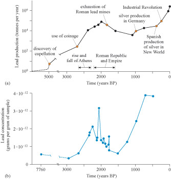
It is important that you look closely at the axes of a graph to make sure that you understand what is being plotted, and on what scale. Some graphs just show the general trend; others may show individual points, with or without connecting lines. Where connecting lines are drawn, as in Figure 11(b), the effect may be to lead your eyes to think that an isolated point is more important than it really is. The visual impact of a graph is both a strength and a weakness!
Activity 4 Taking readings from a graph
From the graph in Figure 11(a), what was the maximum global lead production in tonnes per year before the Industrial Revolution? When did this occur, and what was the lead concentration in the Greenland ice core at this time?
Answer
The peak in global lead production before the Industrial Revolution was approximately 2000 years before the present (BP). At this point, the global lead production was about 105 tonnes per year. The concentration of lead in the Greenland ice core at this time was approximately 3 × 10–12 grams of lead per gram of ice.
Extracting lead from its ores, and to a lesser extent working the lead into pipes etc. (the word ‘plumbing’ derives directly from the Latin for lead, plumbum, as does its chemical symbol, Pb) results in a discharge of lead-rich dust to the atmosphere. Given the pattern of wind movements shown in Figure 9, it is therefore not surprising that lead should appear in the precipitation over the Arctic for the corresponding period.