

2.1 Changing a dataframe’s index
We have seen that by default every dataframe has an integer index for its rows which starts from 0.
The dataframe we’ve been using, london , has an index that goes from 0 to 364 . The row indexed by 0 holds data for the first day of the year and the row indexed by 364 holds data for the last day of the year. However, the column 'GMT' holds datetime64 values which would make a more intuitive index.
Changing the index to datetime64 values is as easy as assigning to the dataframe’s index attribute the contents of the 'GMT' column, like this:
In []:
london.index = london['GMT']
#Display the first 2 rows
london.head(2)
Out[]:
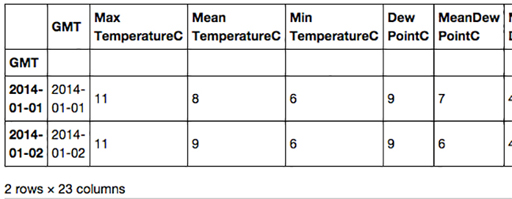
Note that the right of the table has been cropped to fit on the page.
Notice that the 'GMT' column still remains and that the index has been labelled to show that it has been derived from the 'GMT' column.
You can still access a row using the iloc attribute, so to get the first line in the dataframe you can simply execute:
In []:
london.iloc[0]
Out[]:
GMT 2014-01-01 00:00:00
Max TemperatureC 11
Mean TemperatureC 8
Min TemperatureC 6
Dew PointC 9
MeanDew PointC 7
Min DewpointC 4
Max Humidity 94
Mean Humidity 86
Min Humidity 73
Max Sea Level PressurehPa 1002
Mean Sea Level PressurehPa 993
Min Sea Level PressurehPa 984
Max VisibilityKm 31
Mean VisibilityKm 11
Min VisibilitykM 2
Max Wind SpeedKm/h 40
Mean Wind SpeedKm/h 26
Max Gust SpeedKm/h 66
Precipitationmm 9.91
CloudCover 4
Events Rain
WindDirDegrees 186
Name: 2014-01-01 00:00:00, dtype: object
But now you can now also use the datetime64 index to get a row using the dataframe’s loc attribute, like this:
In []:
london.loc[datetime(2014, 1, 1)]
Out[]:
GMT 2014-01-01 00:00:00
Max TemperatureC 11
Mean TemperatureC 8
Min TemperatureC 6
Dew PointC 9
MeanDew PointC 7
Min DewpointC 4
Max Humidity 94
Mean Humidity 86
Min Humidity 73
Max Sea Level PressurehPa 1002
Mean Sea Level PressurehPa 993
Min Sea Level PressurehPa 984
Max VisibilityKm 31
Mean VisibilityKm 11
Min VisibilitykM 2
Max Wind SpeedKm/h 40
Mean Wind SpeedKm/h 26
Max Gust SpeedKm/h 66
Precipitationmm 9.91
CloudCover 4
Events Rain
WindDirDegrees 186
Name: 2014-01-01 00:00:00, dtype: object
A query such as ‘Return all the rows where the date is between 8 December and 12 December’ which you did before (and can still do) with:
In []:
london[(london['GMT'] >= datetime(2014, 12, 8))
& (london['GMT']
can now be done more succinctly like this:
In []:
london.loc[datetime(2014,12,8) : datetime(2014,12,12)]
#The meaning of the above code is get the rows between
#and including the indices datetime(2014,12,8) and
#datetime(2014,12,12)
Out[]:
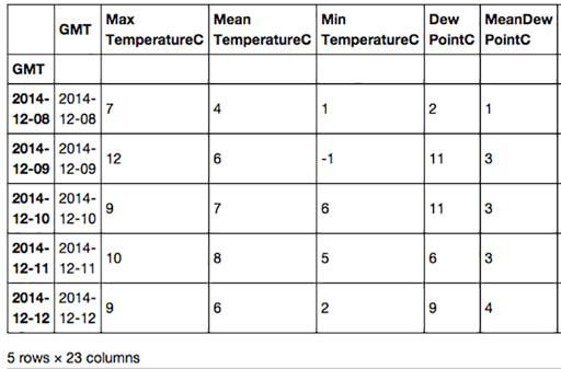
Note that the right of the table has been cropped to fit on the page.
Because the table is in date order, we can be confident that only the rows with dates between 8 December 2014 and 12 December 2014 (inclusive) will be returned. However if the table had not been in date order, we would have needed to sort it first, like this:
london = london.sort_index()
Now there is a datetime64 index, let’s plot ' Max Wind SpeedKm/h 'again:
In []:
london['Max Wind SpeedKm/h'].plot(grid=True, figsize=(10,5))
Out[]:
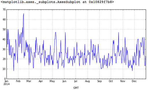
Now it is much clearer that the worst winds were in mid-February.
Exercise 6 Changing a dataframe’s index
Now try Exercise 6 in the Exercise notebook 2.