Climate is a distribution of different types of weather

As well as frequency (i.e. the number of times a particular type of weather occurs), the distribution of weather is also important for climate scientists.

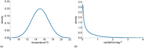
Figure 4 shows another way of expressing the information you saw in Figure 3. But this time, the data are presented as smooth ‘probability distributions. The scale on the vertical y-axis has changed because we have scaled the data so that if you add up all the different measurements of rainfall and temperature, it equals “1”, and the vertical axis is now labelled ‘density’.

Figure 4 Example probability distributions showing invented daily (a) temperature and (b) rainfall

Show description|Hide description

Figure 4a - This is an example probability distribution graph showing one year of invented daily temperature. The x or horizontal axis shows temperature in °C from (8 to 22) °C in steps of 2 °C. The y or vertical axis shows density, from 0.00 to 0.25 in steps of 0.05. The graph is a smooth, bell shaped curve, with a peak in the range (14–15) °C

Figure 4b - This is an example probability distribution graph showing one year of invented daily rainfall. The x or horizontal axis shows rainfall in mm day-1 from (0 to 4) mm day-1. The y or vertical axis shows frequency in days, from 0 to 3.5. The graph is a smooth curve, decreasing exponentially from a maximum where rainfall = 0 mm day-1 to zero at 4 mm day-1.

Figure 4 Example probability distributions showing invented daily (a) temperature and (b) rainfall

From the so called ‘probability density’ we can work out how many occurrences we should expect of things happening. For example, you saw in Figure 4 the density at 14°C temperature was approximately 0.18. But because there was one measurement per day in the data set, the distribution is made up of 365 measurements. So,

The number of times we expect to get a temperature of 14°C = number of measurements* probability density

The number of times we expect to get a temperature of 14°C = 365 * 0.18 = 65.7

And you can see in the figure, the height of the bar is approximately 65.

As well as representing actual data, the shape of the distributions in the figure could equally represent a climate scientist’s judgement as to the probability of temperature or rainfall in the future. The better the scientist’s knowledge or skill, the more likely the distribution is to be correct.

Judgement is formed from a variety of sources of information such as data, theory, computer models, past experience and discussion with others. It might also include educated guesswork. Both data and judgement are used in climate science.