Introduction to active galaxies
Use 'Print preview' to check the number of pages and printer settings.
Print functionality varies between browsers.
Printable page generated Sunday, 22 February 2026, 12:06 PM
Introduction to active galaxies
Introduction
Active galaxies provide a prime example of high-energy processes operating in the Universe. This course introduces the evidence for activity from the spectra of some galaxies, and the concept of a compact active galactic nucleus as a unifying model for the observed features of several types of active galaxy. It also develops the key skill of applying arithmetic and simple algebra to solving scientific problems.
This OpenLearn course is an adapted extract from the Open University course S282 Astronomy.
Learning outcomes
After studying this course, you should be able to:
explain how and why the optical spectrum of an active or starburst galaxy differs from that of a normal galaxy
explain how and why the broadband spectrum of an active or starburst galaxy differs from that of a normal galaxy
describe briefly the observed features of starburst galaxies and the four main classes of active galaxies (quasars, radio galaxies, Seyfert galaxies and blazars)
understand the evidence that indicates the presence of a compact active galactic nucleus (AGN) in active galaxies
explain why an AGN should emit broad lines, narrow forbidden lines and continuous radiation.
1 Overview
Even in images taken with the most modern equipment on a large telescope, it can be difficult to pick out the galaxies now known as 'active' from the other more normal galaxies. But if your telescope were equipped to examine the spectra of the galaxies, then the active galaxies would stand out. Normal galaxies contain stars that are generally similar to those in our own Galaxy; and spiral galaxies have additional similarities to the Milky Way in their gas and dust content. Active galaxies show extra emission of radiation, and this is most apparent from the spectra.
Active galaxies come in a variety of types, including Seyfert galaxies, quasars, radio galaxies and blazars. These types were discovered separately and at first seemed quite different, but they all have some form of spectral peculiarity. There is also evidence in each case that a very large amount of energy is being released in a region that is tiny compared with the size of the galaxy, and so they are classified together. It is usually found that the tiny source region can be traced to the nucleus of the galaxy, so the origin of the excess radiation is attributed to the active galactic nucleus or AGN. An active galaxy may be regarded as a normal galaxy plus an AGN with its attendant effects.
Active galaxies seem to be quite rare in the nearby Universe. Whether every galaxy goes through an active phase in its lifetime, or whether active galaxies are a separate class of object is not clear. We have been aware of these objects only since the 1940s, and the galaxies have been around for at least 1010 years. So the fact that we observe a small percentage of galaxies in an active phase could mean that every galaxy becomes active for the same small percentage of its lifetime, but it could also mean that a small proportion of galaxies become active for a longer time. At present we cannot tell which of these scenarios may be correct. A further complication is that some nearby galaxies, including our own, show evidence of a low level of activity in their nuclei, but we shall concentrate in this course on the prominent and powerful active galaxies.
The engine that powers the AGN, the tiny nucleus of the active galaxy, is a great mystery. It has to produce 1011 or more times the power of our own Sun, but it has to do this in a region little larger than the Solar System. To explain this remarkable phenomenon, a remarkable explanation is required. This has proved to be within the imaginative powers of astronomers, who have proposed that the engine consists of an accreting supermassive black hole, around which gravitational energy is converted into electromagnetic radiation.
In Section 2 you will learn how spectroscopy can be used to distinguish different kinds of galaxy and to measure their properties. Section 3 then introduces the four main classes of active galaxies and describes how they can be recognized. Section 4 examines the evidence for the existence of black holes at the centres of active galaxies, and in Section 5 you will study a simple model that attempts to explain the key characteristics of active galaxies in an illuminating way. Finally, in Section 6, we consider some of the outstanding questions about the origin and evolution of active galaxies.
We begin by looking at the spectra of galaxies.
2 The spectra of galaxies
2.1 What contributes to the spectra of galaxies?
This section reviews what you may already know about the spectra of galaxies. The topic will later be developed further to help you appreciate the spectra of active galaxies.
The four main constituents of a galaxy are dark matter, stars, gas and dust.
Even though dark matter is the main constituent of a galaxy, it does not contribute to the spectrum of the galaxy so we need not consider it any further. The spectrum of a galaxy contains contributions from stars, gas and (sometimes) dust.
The spectrum of a star normally consists of a continuous thermal spectrum with absorption lines cut into it (Figure 1). It is possible to learn a lot about the star from a study of these absorption lines.
What can be learned about a star from its absorption lines? The strengths and widths of the absorption lines contain information about the star's chemical composition, surface temperature and luminosity. By looking for Doppler shifts in the lines you can measure radial velocity and, if the Doppler shifts are periodic in time, you can detect the binary nature of a star.
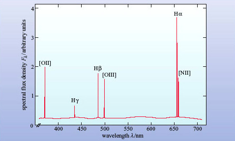
The gas in a galaxy is partly visible in the form of hot clouds known as HII regions. Such regions are usually only seen where there is ongoing star formation, and so are prominent in spiral and irregular galaxies. The optical spectrum of an HII region consists of just a few emission lines, as can be seen in Figure 2. HII regions can make a substantial contribution to the spectra of galaxies because they are very bright. The only other gaseous objects in a normal galaxy to emit at optical wavelengths are supernova remnants and planetary nebulae, and these are faint compared with HII regions.
The dust component of a galaxy, being relatively cool, does not lead to any emission features in the optical spectrum of a galaxy. The main effect of dust at optical wavelengths is to absorb starlight. However, dust can emit strongly at far-infrared wavelengths (λ of about 100 μm).
As a rule, optical absorption lines result from stars, and optical emission lines result from hot gas.
The spectra of stars and HII regions extend far beyond the optical region. The Sun, for example, radiates throughout the ultraviolet, X-ray, infrared and radio regions of the electromagnetic spectrum. The majority of the Sun's radiation is concentrated into the optical part of its spectrum but, as you will shortly see, this is not the case for active galaxies, for which it is necessary to consider all the observed wavelength ranges. We shall call this the broadband spectrum to distinguish it from the narrower optical spectrum.
The word optical means visible wavelengths plus the near ultraviolet and near infrared wavelengths that can be observed from the ground, and extends from 300 to 900 nm. The optical spectrum is just one part of the broadband spectrum albeit an important part. The spectrum of a normal galaxy is the composite spectrum of the stars and gas that make up the galaxy. Some of the absorption lines of the stars and some of the emission lines of the gas can be discerned in the galaxy's spectrum. As well as being able to work out the mix of stars that make up the galaxy, astronomers can measure the Doppler shifts of these spectral lines and so work out the motions within the galaxy as well as the speed of the galaxy through space.
In the case of active galaxies, the spectrum shows features in addition to those of normal galaxies, and it is from these features that the active nucleus of the galaxy can be detected.
2.2 Optical spectra
2.2.1 Normal galaxies
Normal galaxies are made up of stars and (in the case of spiral and irregular galaxies) gas and dust. Their spectra consist of the sum of the spectra of these components.
The optical spectra of normal stars are continuous spectra overlaid by absorption lines (Figure 1). There are two factors to consider when adding up the spectra of a number of stars to produce the spectrum of a galaxy:
Different types of star have different absorption lines in their spectra. When the spectra are added together, the absorption lines are 'diluted' because a line in the spectrum of one type of star may not appear in the spectra of other types.
Doppler shifts can affect all spectral lines. All lines from a galaxy share the red-shift of the galaxy, but Doppler shifts can also arise from motions of objects within the galaxy. As a result, the absorption lines become broader and shallower. We explain below how this Doppler broadening comes about.
HII regions in spiral and irregular galaxies (though not, of course, ellipticals) shine brightly and contribute significantly to the spectrum of the galaxy. The optical spectrum of an HII region consists mainly of emission lines, as in Figure 2. When the spectra of the HII regions and the stars of a galaxy are added together, the emission lines from the HII regions tend to remain as prominent features in the spectrum unless a line coincides with a stellar absorption line. There are Doppler shift effects, however, as described for stellar absorption lines, and hence emission lines too are broadened because of the motion of HII regions within a galaxy.
Box 1: Doppler Broadening
The Doppler effect causes wavelengths to be lengthened when the source is moving away from the observer (red-shifted) and shortened when the source is moving towards the observer (blue-shifted).
Light from an astrophysical source is the sum of many photons emitted by individual atoms. Each of these atoms is in motion and so their photons will be seen as blue- or red-shifted according to the relative speeds of the atom and the observer. For example, even though all hydrogen atoms emit H![]() photons of precisely the same wavelength, an observer will see the photons arrive with a spread of wavelengths: the effect is to broaden the H
photons of precisely the same wavelength, an observer will see the photons arrive with a spread of wavelengths: the effect is to broaden the H![]() spectral line - called Doppler broadening.
spectral line - called Doppler broadening.
In general, if the emitting atoms are in motion with a range of speeds Δν along the line of sight to the observer (the velocity dispersion) then the Doppler broadening is given by

where c is the speed of light, and λ is the central wavelength of the spectral line.
Why would the atoms be in motion? An obvious reason is that they are 'hot'. Atoms in a hot gas, for example, will be moving randomly with a range of speeds related to the temperature of the gas. For a gas of atoms of mass m at a temperature T, the velocity dispersion is given by

where k is the Boltzmann constant (1.38 × 10⁻²³ J K−1).
Question 1
Calculate the velocity dispersion for hydrogen atoms in the solar photosphere (temperature ∼6 × 10³ K). Then work out the width in nanometres of the H![]() line (656.3 nm) due to thermal Doppler broadening.
line (656.3 nm) due to thermal Doppler broadening.
Answer
For the Sun's photosphere we have T = 6000 K and m = mH = 1.67 × 10⁻²⁷ kg.
So the velocity dispersion is given by
So hydrogen atoms in the Sun's atmosphere are moving at around 10 km s−1.
Rearranging Equation 3.1 we have
so the Doppler broadening of the solar H![]() line is 0.02 nm (to 1 significant figure). (This is a tiny broadening, about 1 part in 30 000, and rather difficult to observe.)
line is 0.02 nm (to 1 significant figure). (This is a tiny broadening, about 1 part in 30 000, and rather difficult to observe.)
It is very common for Doppler broadening to be expressed as a speed rather than Δλ or even Δλ/λ. So astronomers would say that the width of the solar H![]() line is about 10 km s−1.
line is about 10 km s−1.
You can also see that thermal Doppler broadening depends on the mass of the atom so, for the same temperature, hydrogen lines will be wider than iron lines.
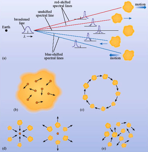
Thermal motion is not the only way in which a velocity dispersion can arise. Bulk movements of material can also broaden spectral lines.
What kinds of bulk motions could give rise to Doppler broadening?
For a line to be broadened, the emitting atoms must be moving at different speeds along the line of sight. This could occur where a gas cloud is rotating, where gas is flowing inwards or outwards from a centre, or where gas is in turbulent or chaotic motion.
So a galaxy rotating about its centre will produce a spectrum in which the lines are broadened. Normal galaxies have Δν values of between 100 and 300 km s−1, which you can see is far higher than thermal motions in a hot gas such as the Sun's photosphere. Whether the bulk motion is a rotation, an infall, an outflow, or just turbulence makes no difference; the net effect will be a broadened line whose width is proportional to the range of velocities present.
How might you distinguish thermal broadening in a spectrum from broadening due to bulk motions?
Thermal broadening depends on the mass of the individual emitting atoms (heavy atoms move more slowly) so lines from different elements will have different values of Δλ/λ. Broadening from bulk motion will affect all spectral lines equally; they will have the same value of Δλ/λ.
Doppler broadening applies equally to emission and absorption lines. The broadening is due to the motion of the emitting or absorbing atoms (Figure 3).
Question 2
Our Galaxy rotates at between roughly 200 and 250 km s−1. Estimate the broadening of lines if it were observed edge-on by an astronomer situated in a distant cluster of galaxies. (Assume that our Galaxy is not spatially resolved in such observations.)
Answer
Edge-on, this is the approach speed at one extremity and the recession speed at the other. So the line-width that would be observed if the Galaxy were viewed edge-on is 400-500 km s−1.
One more feature of emission lines from HII regions needs to be mentioned, and that is the presence of so-called forbidden lines, as opposed to the others, which are called permitted lines. The term 'forbidden line' arose from quantum theory. The permitted lines all obey a certain set of rules in that theory, whereas the forbidden lines break these rules. Most spectral lines that are seen astronomically can be produced in regions of either high or low gas density. Forbidden lines are produced only in regions of very low density; this is because the excited states responsible for their production are so long-lived that, at higher densities, the atom or ion is likely to be de-excited by collision with another particle before a photon can be emitted spontaneously. Such low densities cannot be achieved on Earth which is why these lines are not observed in the laboratory. When they are observed astronomically, we can be sure that they have been produced in a region of extremely low density. They are prominent in the spectra of active galaxies and are denoted by square brackets [ ]. Strong forbidden lines seen in HII regions include [NII] at 655nm and [OIII] at 501 nm (see Figure 2).
So what will the spectrum from a normal galaxy look like? It depends what kind of galaxy it is. The optical spectrum of an elliptical galaxy is a continuous spectrum with absorption lines. Sensitive observations of elliptical galaxies typically reveal the presence of many absorption lines, although these lines are somewhat broader and shallower than those seen in individual stellar spectra. There are no emission lines, because elliptical galaxies have no HII regions. The overall shape of the spectrum looks like that of a K-type (fairly cool) star because cool giant stars dominate the luminous output of the galaxy.
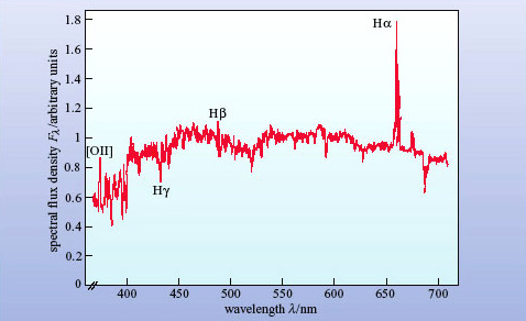
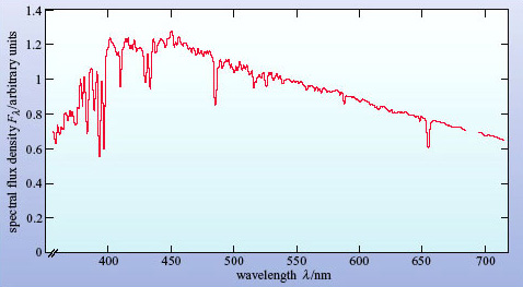
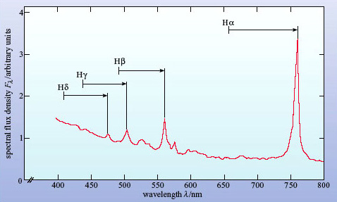
The optical spectrum of a spiral galaxy consists of the continuous spectrum from starlight with a few shallow absorption lines from stars, plus a few rather weak emission lines from the HII regions. Figure 4 shows an example. Note that the H![]() line in this spectrum is a result of both absorption from stars and emission from HII regions.
line in this spectrum is a result of both absorption from stars and emission from HII regions.
Why has there been no mention of dust so far?
Because we are only discussing optical spectra. Other than dimming the starlight, dust has no emission or absorption lines in the optical region.
Before moving on to consider the spectrum of active galaxies, look at the spectrum in Figure 5.
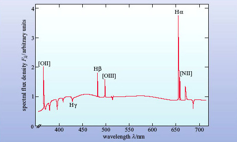
How does the spectrum of the mystery galaxy in Figure 5 compare with those in Figure 2 and Figure 4? How would you interpret the difference?
The spectrum in Figure 5 shows very strong emission lines, similar to the spectrum of an HII region in Figure 2. Although the stellar absorption spectrum is present, the line spectrum is dominated by HII regions rather than stars. It looks like a galaxy with more HII regions than normal.
In fact, Figure 5 is the spectrum of a starburst galaxy. Starburst galaxies are otherwise normal galaxies that are undergoing an intense episode of star formation. They contain many HII regions illuminated by hot, young stars, and the emission lines show up clearly in the optical spectrum. We mention starburst galaxies here because, as you will see, their spectra have a resemblance to active galaxies, and it is important to be able to distinguish them.
Active galaxies
Figure 6 shows a schematic optical spectrum of an active galaxy. It is immediately apparent that the emission lines are stronger and broader than in the spectrum of a normal galaxy shown in Figure 4. They are also broader than in the spectrum of the starburst galaxy in Figure 5. It is as if a component producing strong and broad emission lines had been added to the spectrum of Figure 4.
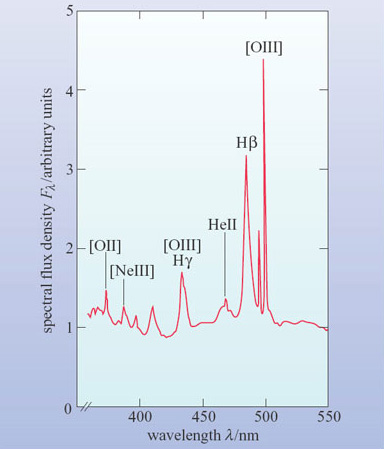
From what you have learned so far, what might be the nature of this component?
The strong emission lines suggest that the galaxy contains hot gas similar to an HII region. The broad lines imply that the gas must be either extremely hot or in rapid motion.
Now answer Question 3, which will help you decide which of these two possibilities is the more likely.
Question 3
Measure the wavelength and width of the Hβ line in Figure 6 (at half the height of the peak above the background) and so make a rough calculation of the velocity dispersion of the gas that gave rise to it. If the line widths are due to thermal Doppler broadening, estimate the temperature of the gas.
Answer
The Hβ line has a wavelength of about 485 nm and a width of roughly 6 nm. So the velocity dispersion is
Rearranging Equation 3.2 and putting m = mH we have
In view of the difficulty of measuring the width of the line, it would be appropriate to give the temperature as approximately 109 K. (As is explained in the text following this question, the Hβ emitting region does not have such a high temperature.)
The answer to Question 3 is quite surprising. Not only is the implied temperature higher than the core temperatures of all but the most massive stars, it is also inconsistent with the process by which H![]() emission occurs, since at such temperatures any hydrogen would be completely ionized. In fact, the relative strengths of various emission lines can be used to estimate the temperature of the gas, and this is found to be only about 104 K. So the broadening cannot be thermal.
emission occurs, since at such temperatures any hydrogen would be completely ionized. In fact, the relative strengths of various emission lines can be used to estimate the temperature of the gas, and this is found to be only about 104 K. So the broadening cannot be thermal.
The alternative explanation is bulk motions of several thousand kilometres per second. These are very large velocities indeed, and imply that large amounts of kinetic energy are tied up in the gas motions. We shall return to the nature of these motions later in this course.
2.3 Broadband spectra
The broadband spectrum is the spectrum over all the observed wavelength ranges. To plot the broadband spectrum of any object it is necessary to choose logarithmic axes.
Why is it necessary to use logarithmic axes?
Because both the spectral flux density, Fλ, and the wavelength vary by many powers of 10.
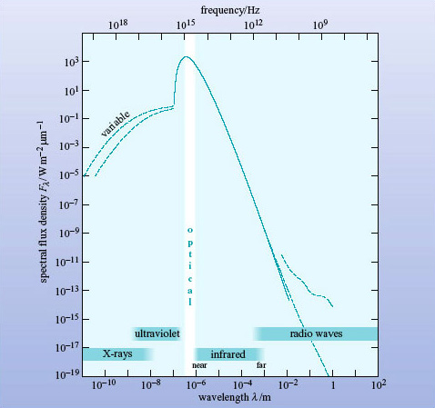
Figure 7 shows the broadband spectrum of the Sun: it has a strong peak at optical wavelengths with very small contributions at X-ray and radio wavelengths.
Normal galaxies
Figure 8 shows schematically the broadband spectrum of a normal spiral galaxy. It resembles that of the Sun, although the peak occurs at a slightly longer wavelength and there are relatively greater spectral flux densities at X-ray, infrared and radio wavelengths.
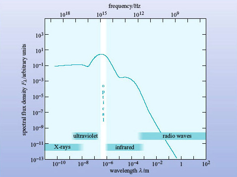
What are the objects in a normal galaxy that emit at (a) X-ray, (b) infrared and (c) radio wavelengths?
(a) X-rays are emitted by X-ray binary stars, supernova remnants and the hot interstellar medium.
(b) Infrared radiation comes predominantly from cool stars, dust clouds, and dust surrounding HII regions.
(c) Radio waves are emitted by supernova remnants, atomic hydrogen and molecules such as CO.
From Figure 8 you would conclude that the spectrum peaks in the optical, but there is a subtlety in the definition of Fλ which needs to be addressed.
Look again at the broadband spectrum in Figure 8. Is this galaxy brighter in X-rays or in the far-infrared (λ ∼ 100 μm)?
The Fλ curve is higher in the X-ray region, so the galaxy appears to be brighter in X-rays than in the far-infrared (far-IR).
Obvious, isn't it? Well, appearances can be misleading. The spectral flux density Fλ is defined as the flux density received over a 1-μm bandwidth (see Box 2). At far-IR and radio wavelengths that bandwidth is a tiny fraction of the spectrum. But at shorter wavelengths, 1 μm covers the entire X-ray, UV and visible regions of the spectrum! So Fλ will underestimate the energy emitted by a galaxy in the far-IR (and radio wavelengths) and exaggerate the energy emitted in X-rays.
To correct this bias in Fλ spectra, astronomers often plot the quantity λFλ instead. λFλ, pronounced 'lambda eff lambda', (with units of W m−2) is a useful quantity when we are comparing widely separated parts of a broadband spectrum. If the spectrum in its normal form of Fλ against λ is replotted in the form of λFλ against λ, (still on logarithmic axes) then the highest points of λFλ will indicate the wavelength regions of maximum power received from the source.
A broadband spectrum plotted in this way is known as a spectral energy distribution (or SED) because the height of the curve is a measure of the energy emitted at each point in the spectrum.
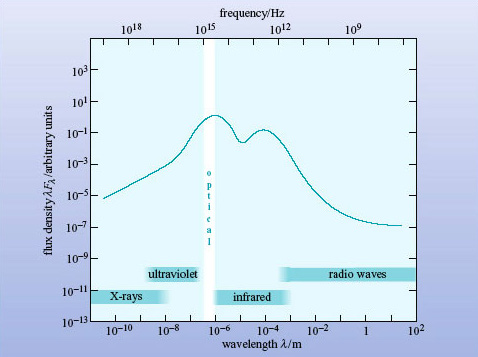
In Figure 9, λFλ has been plotted against λ for the normal galaxy spectrum of Figure 8, and it can be clearly seen that this curve has a peak at optical wavelengths, confirming what was suspected. But it also shows that more energy is being radiated at far-IR wavelengths than in X-rays, the opposite of the impression given by Figure 8. From now on in this course broadband spectra will be plotted as SEDs with λFλ against λ on logarithmic axes.
You may have found the concept of λFλ difficult to grasp. If so, don't worry about the justification, but just accept that a λFλ plot allows you to compare widely differing wavelengths fairly, whereas a conventional Fλ plot does not.
Box 2: Flux Units
Astronomers use several different units to measure the electromagnetic radiation received from an object.
Flux density, F, is the power received per square metre of telescope collecting area. It is measured in watts per square metre, W m−2.
Spectral flux density is the flux density measured in a small range of bandwidth. As bandwidth can be expressed either in terms of wavelength (λ) or frequency (ν) there are two kinds of spectral flux density in common use.
Fλ is measured in watts per square metre per micrometre (W m−2 μm−1) and Fv is measured in watts per square metre per hertz (W m−2 Hz−1). The former is preferred by optical and infrared astronomers (who work in wavelengths) and the latter by radio astronomers (who work in frequencies). The special course, the jansky (Jy), is given to a spectral flux density of 10−26 W m−2 Hz−1, in honour of the US engineer Karl Jansky (1905-1950) who made pioneering observations of the radio sky in the early 1930s.
Both flux density and spectral flux density are commonly (though inaccurately) referred to as flux.
Note that the symbol ν (Greek letter 'nu') is commonly used to denote the frequency of electromagnetic radiation. In this course, the convention is to use f to denote frequency.
Question 4
Astronomers observe two galaxies at the same distance. Both have broad, smooth spectra.
Galaxy A is seen at optical wavelengths (around 500 nm), and yields a spectral flux density Fλ = 10−29 W m−2 μm−1; it is not detected in the far infrared at around 100 μm (the upper limit to the measured flux density is Fλ < 10−32 W m−2 μm−1).
Galaxy B appears fainter in the optical and gives Fλ = 10−30 W m−2 μm−1 around 500 nm, and the same value at around 100 μm.
Which (on these data) is the more luminous galaxy?
Answer
In the optical region (λ = 0.5 μm) galaxy A has λFλ = 0.5 × 10⁻²⁹ W m−2.
For galaxy B, λFλ = 0.5 × 10⁻³⁰ W m−2.
So galaxy A is 10 times brighter in the optical.
In the far-infrared (λ = 100 μm), the upper limit to λFλ is 10−30 W m−2 whereas galaxy B has λFλ = 10−28 W m−2. The far-infrared flux density of galaxy B is not only greater than that of galaxy A at this wavelength, but also exceeds the flux density at optical wavelengths of both galaxies. On the basis of these (very sparse!) data, it is concluded that galaxy B is the more luminous galaxy.
Active galaxies
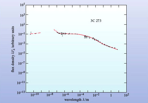
Figure 10 shows the spectral energy distribution of an active galaxy.
In broad terms, what is the major difference between the SED of the normal galaxy in Figure 9 and the SED of the active galaxy in Figure 10?
Compared with the (unquantified) peak emission, the SED of the active galaxy is much flatter than that of the normal spiral galaxy. This indicates that there is relatively much more emission (by several orders of magnitude) at X-ray wavelengths and at radio wavelengths.
For the active galaxy (known from its catalogue number as 3C 273) the peak emission is in the X-ray and ultraviolet regions. Many other active galaxies are bright in this region and the feature is known as the 'big blue bump'. In some active galaxies, though not this one, the infrared emission is prominent. These galaxies emit a normal amount of starlight in the optical, so they must emit several times this amount of energy at infrared and other wavelengths - this is another feature that distinguishes active galaxies from normal galaxies. It means that we have to account for several times the total energy output of a normal galaxy, and possibly a great deal more. A normal galaxy contains 1010 to 1011 stars, so we need an even more powerful energy source for active galaxies.
The term spectral excess is used (rather loosely) to refer to the prominence of infrared or other wavelength regions in the broadband spectra of active galaxies. In particular, it is often used to indicate the presence of emission in a certain wavelength region that is over and above that which would be expected from the stellar content of a galaxy.
Question 5
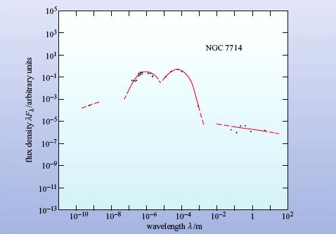
Now that you have some experience in interpreting the spectra of galaxies, look at the SED of the galaxy NGC 7714 in Figure 11. Describe as fully as you can what the diagram tells you about this galaxy. Can you guess what sort of galaxy it is?
Answer
The spectrum shows two distinct peaks, one at the red end of the optical (similar to a normal galaxy) and one far into the infrared, near 100 μm. The far-infrared peak is at a similar wavelength to the small peak in a normal spiral galaxy, but it is higher than the optical peak, suggesting that this galaxy emits most of its energy in the far-infrared. There is no significant emission in the UV or X-ray region.
This is not a normal galaxy and you might have guessed that it is an active galaxy. In fact, it is a starburst galaxy. The infrared radiation is coming from dust heated by the continuing star formation and is another distinguishing characteristic of a starburst galaxy, in addition to the strong narrow optical emission lines that you encountered earlier.
3 Types of active galaxies
3.1 Introduction
Active galaxies have occupied the attention of an increasing number of astronomers since the first example was identified in the 1940s. By one recent estimate, a fifth of all research astronomers are working on active galaxies, which indicates how important this field is. In this section you will learn about the observational characteristics of the four main classes of active galaxies: Seyfert galaxies, quasars, radio galaxies and blazars. This will set the scene for subsequent sections in which we will explore the physical processes that lie behind these different manifestations of active galaxies.
3.2 Seyfert galaxies
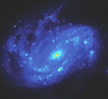
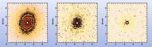
In 1943 the American astronomer Carl Seyfert (1911-1960) drew attention to a handful of spiral galaxies that had unusually bright point-like nuclei. Figure 12 shows NGC 4051, one of the first Seyfert galaxies to be identified. Subsequently, it has been found that compared to normal galaxies, Seyfert galaxies show an excess of radiation in the far infrared and at other wavelengths. Even more remarkably, at some wavelengths, including the optical, this excess radiation is variable. The variability implies that the emission from a Seyfert galaxy must come from a region that is tiny compared to the galaxy itself.
Spectra of the bright nuclei reveal that Seyferts can be classified into two types by the relative widths of their emission lines (Figure 13).
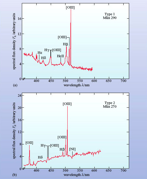
Type 1 Seyferts have two sets of emission lines (Figure 13a). The narrower set, which are made up largely of the forbidden lines discussed earlier, have widths of about 400 km s−1. Despite this considerable width the region emitting these lines is known as the narrow-line region. The broader lines, consisting of permitted lines only, have widths up to 10 000 km s−1 and appear to originate from a denser region of gas known as the broad-line region.
Forbidden lines are sensitive to the gas density in the emitting region. An analysis of which lines are present allows the densities of the gas in the broad- and narrow-line regions to be determined. These two regions are also characteristic of other types of active galaxy. Type 2 Seyferts only show prominent narrow lines (Figure 13b). The broad lines are either absent or very weak in the optical spectra of type 2 Seyferts.
In fact, these two types are not as clear cut as they first seemed, since weak broad lines have now been found in Seyferts previously classed as type 2. Types 1 and 2 are better understood as extreme ends of a range of intermediate Seyfert types classified according to the relative strengths of their broad and narrow lines. In a Seyfert 1.5, for example, there are broad and narrow lines, but the broad lines are not as strong as those seen in type 1 Seyferts.
Box 3: Carl Keenan Seyfert (1911-1960)
Carl Seyfert (Figure 14) was born and grew up in Cleveland, Ohio. He entered Harvard with the intention of studying medicine, but became diverted from this career path after attending an inspirational lecture course in astronomy given by Bart Bok. Seyfert switched his attention to astronomy and remained at Harvard to carry out his doctoral research under the direction of Harlow Shapley.
Following a post at Yerkes Observatory he was employed at Mount Wilson Observatory from 1940 to 1942. It was during this time at Mount Wilson that he carried out his observations into the type of galaxies that now carry his name. During the Second World War he managed to juggle several tasks: teaching navigation to the armed forces, carrying out classified research, and still finding time to partake in some astronomical research. He is notable for producing some of the first colour photographs of nebulae and stellar spectra - some of which were used in the Encyclopedia Britannica.
After the war Seyfert gained a faculty position at Vanderbilt University in Nashville, Tennessee. He was the driving force behind the development of their observatory and was also an enthusiastic popularizer of science. He also found time to present local weather forecasts on television! He was tragically killed in a motor accident in 1960 at the age of 49. He died before the significance of Seyfert galaxies became fully apparent - the field of active galaxy research only became a key area of astronomy after the discovery of quasars in 1963.
3.3 Quasars
One of the most unexpected turns in the history of astronomy was the discovery of quasars. When first recognised, in 1963, quasars appeared at radio and optical wavelengths as faint, point-like objects with unusual optical emission spectra. The name comes from their alternative designations of 'quasi-stellar radio source' (QSR) or 'quasi-stellar object' (QSO), meaning that they resemble stars in their point-like appearance. Their spectra, however, are quite unlike those of stars. The emission lines turn out to be those of hydrogen and other elements that occur in astronomical sources, but they are significantly red-shifted.
Figure 15 shows the optical spectrum of 3C 273, which was the first quasar to be discovered (you have already seen its broadband spectrum in Figure 10). The redshift is 0.158, which corresponds to a distance of about 660 Mpc according to Hubble's law. Many other quasars are now known - a recent catalogue lists more than 7000 - and the vast majority have even greater redshifts, the record (in 2003) being more than 6. All quasars must therefore be highly luminous to be seen by us at all.
The optical spectra of quasars are similar to those of Seyfert 1 galaxies, with prominent broad lines but rather weaker narrow lines. A composite spectrum for 700 quasars is shown in Figure 16. To form this spectrum, the individual quasar spectra were all corrected to remove the effect of red-shift before being added together. Because many quasars have high redshifts, many of the features that are observed in the visible part of the spectrum correspond to emission features in the ultraviolet. In particular, the spectrum shows the Lyman ![]() (Ly
(Ly![]() ) line that arises from the electronic transition in atomic hydrogen from the state n = 2 to n = 1. This line, which occurs at a wavelength of 121.6 nm, is clearly a very strong and broad line in quasar spectra.
) line that arises from the electronic transition in atomic hydrogen from the state n = 2 to n = 1. This line, which occurs at a wavelength of 121.6 nm, is clearly a very strong and broad line in quasar spectra.
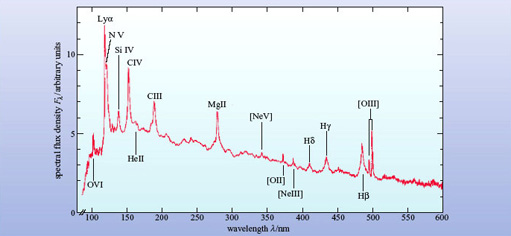
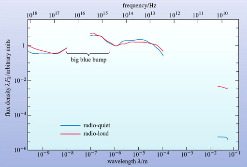
Quasars show spectral excesses in the infrared and at other wavelengths. About 10% of quasars are strong radio sources and are said to be radio loud. Some astronomers prefer to retain the older term QSO (quasi-stellar object) for radio-quiet quasars that are not strong sources of radio waves. The spectral energy distribution for a sample of radio-loud and a sample of radio-quiet quasars is shown in Figure 17. The big blue bump, hinted at in Figure 10, is particularly prominent here. Many quasars are also variable throughout the spectrum on timescales of months or even days.
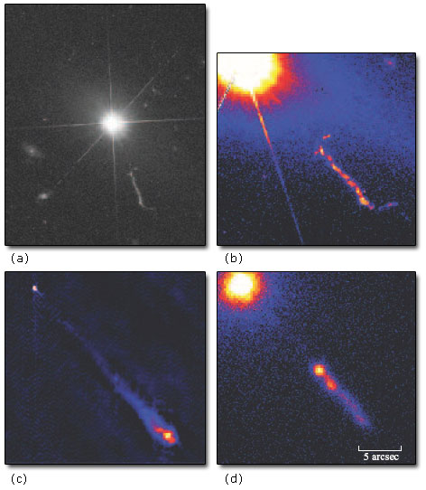
Detailed radio mapping shows that many of the radio-loud quasars have prominent jets which appear to be gushing material into space. In 3C 273 the jet is even visible on optical images (Figure 18).
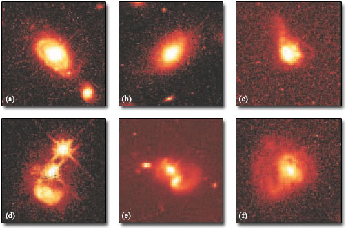
Because quasars are so distant, it has been difficult to study the host galaxies which contain them. Recent work seems to show that there is no simple relationship between a quasar and the morphology of its host galaxy - while many quasar host galaxies are interacting or merging systems, there are also many host galaxies that appear to be normal ellipticals or spirals (Figure 19). It has also been found that the radio-loud quasars tend to be found in elliptical and interacting galaxies whereas the radio-quiet quasars (the QSOs) seem to be present in both elliptical and spiral host galaxies. It should be stressed however that the relationship between quasar host and radio emission is not clear-cut, and that this is a topic of ongoing research.
Before their host galaxies were discovered in the 1980s quasars seemed much more puzzling than they do now. Indeed, for many years, there was a school of thought that supported the idea that quasars were not at such great distances as they are now thought to be, but were instead relatively close objects in which the red-shift arose from some unknown physical process. The study of quasar host galaxies has all but dispelled this view and the modern picture of a quasar is of a remote, very luminous AGN buried in a galaxy of normal luminosity. This is why astronomers now regard quasars as a type of active galaxy, though you will still see books referring to 'active galaxies and quasars'. Quasars are believed to be the most luminous examples of AGNs known.
3.4 Radio galaxies
Radio galaxies were discovered accidentally by wartime radar engineers in the 1940s, although it took another decade for them to be properly studied by the new science of radio astronomy. Radio galaxies dominate the sky at radio wavelengths. They show enormous regions of radio emission outside the visible extent of the host galaxy - usually these radio lobes occur in pairs.
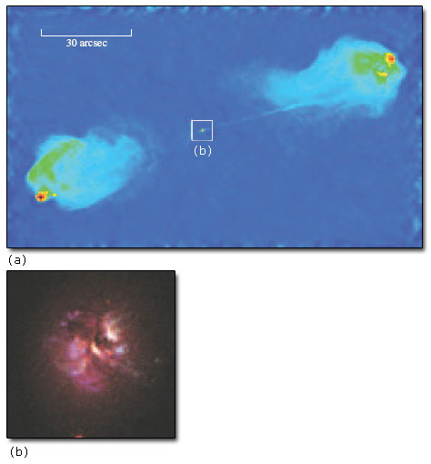
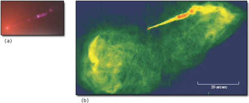
The first radio galaxy to be discovered, and still the brightest, is called Cygnus A (Figure 20). Radio maps show the two characteristic lobes on either side of a compact nucleus. A narrow jet is apparent to the right of the nucleus and appears to be feeding energy out to the lobe. There is a hint of a similar jet on the left. Jets are a common feature of radio galaxies, especially at radio wavelengths. They trace the path by which material is being ejected from the AGN into the lobes.
Cygnus A is an example of the more powerful class of radio galaxy with a single narrow jet. The second jet is faint, or even absent, in many powerful radio galaxies; we will consider the reasons for this shortly. Note the relatively inconspicuous nucleus and the bright edge to the lobes, as if the jet is driving material ahead of it into the intergalactic medium.
The jets of weaker radio galaxies spread out more and always come in pairs. These galaxies have bright nuclei, but the lobes are fainter and lack sharp edges. You can see an example in Figure 21. This is M84, a relatively nearby radio galaxy in the Virgo cluster of galaxies.
Each radio galaxy has a point-like radio nucleus coincident with the nucleus of the host galaxy. It is this feature that is reminiscent of other classes of active galaxies and which is believed to be the seat of the activity. The nucleus shows many of the properties of other AGNs, including emission lines, a broadband spectrum which is far wider than that of a normal galaxy, and variability.
The optical spectrum of the nucleus of a radio galaxy looks very much like that of any other AGN. Like Seyferts, radio galaxies can be classified into two types depending on whether broad lines are present (broad-line radio galaxies) or only narrow lines (narrow-line radio galaxies). Figure 22 shows an example of a spectrum of a broad-line radio galaxy.
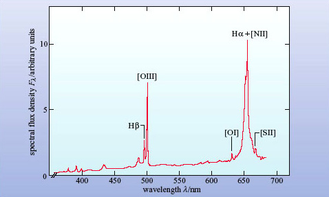
Figure 23 shows maps of radio, optical and X-ray wavelengths of Centaurus A, which is the nearest radio galaxy to the Milky Way. The optical image (Figure 23b) shows that it is an elliptical galaxy with a dust lane bisecting it.
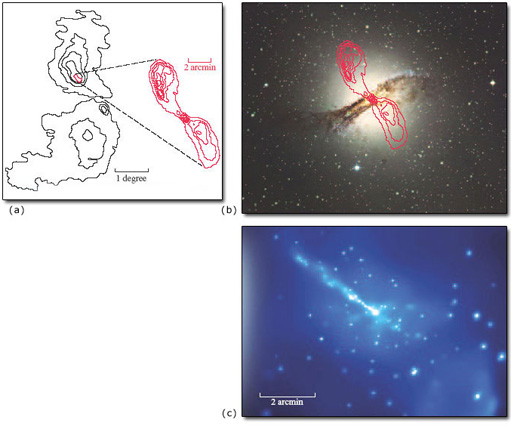
Given that Centaurus A is an elliptical galaxy, does anything strike you as incongruous about Figure 23b?
Elliptical galaxies are supposed to have negligible amounts of dust, so the thick dust lane seems very strange indeed!
The galaxy is obviously not a normal elliptical and this is a clue to the nature of radio galaxies. In fact, it is now thought that Centaurus A was formed by the collision of a spiral galaxy with a massive elliptical, the dust lane being the remains of the spiral's disc. We will come back to this interesting topic later in the course.
M87 (also known as Virgo A) is such a well-known radio galaxy that it must be mentioned at this point. In the optical region it, too, appears as a giant elliptical galaxy at the centre of the nearby Virgo cluster of galaxies. It seems that most radio galaxies are ellipticals. The single bright jet in the galaxy (Figure 24) is reminiscent of the jet in the quasar 3C 273 shown in Figure 18.
3.5 Blazars
Blazars appear star-like, as do quasars, but were only recognised as a distinct class of object in the 1970s. They are variable on timescales of days or less. All are strong and variable radio sources. There are two subclasses.
BL Lac objects are characterised by spectra in which emission lines are either absent or extremely weak. They lie at relatively low redshifts. At first, they were mistaken for variable stars until their spectra were studied. (Their name derives from BL Lacertae which is the variable-star designation originally given to the first object of this type to be studied.)
Just over 100 BL Lacs are known and evidence for host galaxies has been found for 70 or so. Figure 25 shows three examples of a survey of BL Lac host galaxies that was conducted with the Hubble Space Telescope. In most cases the host galaxy appears to be elliptical and the stellar absorption lines help to confirm the redshift of the object.
Optically violent variables (OVVs) are very similar to BL Lacs but have stronger, broad emission lines and tend to lie at higher redshifts.
3.6 A 'non-active' class - the starburst galaxies
We end this section by drawing a distinction between the classes of active galaxy that are described in the previous subsections and the starburst galaxies mentioned earlier. As you have seen, starburst galaxies are essentially ordinary galaxies in which a massive burst of star formation has taken place. Their spectra show emission lines from their many HII regions and infrared emission from dust but, in the main, they do not show unusual activity in their nuclei. In the past they were regarded as active galaxies but modern practice is to place them in a class of their own.
Although it is clear that there are starburst galaxies that are not active galaxies, it does appear that some active galaxies are undergoing a burst of star formation. It is not clear at present whether there is a link between these two types of phenomenon where they are seen in the same galaxy but, as you will see later, it is possible that both types of phenomenon - rapid star formation and activity in the galactic nucleus - may be triggered by galactic collisions and mergers.
Question 6
Take a few minutes to jot down as many differences that you can think of between normal galaxies and each of the four types of active galaxy. Are there any characteristics which all active galaxies have in common?
Answer
There are several things you may have thought of. Table 1 summarises many of the characteristics and includes some pieces of new information as well. What all active galaxies have in common is a powerful, compact nucleus which appears to be the source of their energy.
| Characteristic | Active galaxies | ||||
|---|---|---|---|---|---|
| Normal | Seyfert | Quasar | Radio galaxy | Blazar | |
| Narrow emission lines | weak | yes | yes | yes | no |
| Broad emission lines | no | some cases | yes | some cases | some cases |
| X-rays | weak | some cases | some cases | some cases | yes |
| UV excess | no | some cases | yes | some cases | yes |
| Far-infrared excess | no | yes | yes | yes | no |
| Strong radio emission | no | no | some cases | yes | some cases |
| Jets and lobes | no | no | some cases | yes | no |
| Variability | no | yes | yes | yes | yes |
Activity: the AGN zoo
Open the AGN zoo document linked below and use the online NED database of galaxies to complete the activity as instructed in the document.
Click below 6 pages 0.15 MB
4 The central engine
4.1 Introduction: the active galactic nuclei (AGN)
From Section 3 you will have discovered that one thing all active galaxies have in common is a compact nucleus, the AGN, which is the source of their activity. In this section you will study the two properties of AGNs that make them so intriguing - their small size and high luminosity - and learn about the energy source at the heart of the AGN, the central engine.
4.2 The size of AGNs
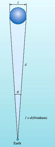
AGNs appear point-like on optical images. It is instructive to work out how small a region these imaging observations indicate. Optical observations from the Earth suffer from 'seeing', the blurring of the image by atmospheric turbulence. The result is that star-like images are generally smeared by about 0.5 arcsec or more. One can do much better with the Hubble Space Telescope where, thanks to the lack of atmosphere, resolved images can be as small as 0.05 arcsec. What does this mean in terms of the physical size of an AGN?
An arc second is 1/3600 of a degree and there are 57.3 degrees in a radian. So 0.05 arcsec corresponds to an angle of 0.05/(57.3 × 3600) rad = 2.4 × 10⁻⁷ rad. For such a small angle, the linear diameter ![]() of an object is related to its distance d by
of an object is related to its distance d by ![]() = d × θ, where θ is its angular diameter in radians (Figure 26).
= d × θ, where θ is its angular diameter in radians (Figure 26).
The nearest known AGN is NGC 4395, a Seyfert at a distance of 4.3 Mpc and it, too, is unresolvable with the Hubble Space Telescope. So its linear size ![]() must be less than (4.3 × 106) × (2.4 × 10−7) pc = 1.0 pc. So, for a nearby AGN, we can place an upper limit of order 1 pc on its linear size. (For a more distant AGN, this upper limit is correspondingly larger.) A parsec is a tiny distance in galactic terms. Even the nearest star to the Sun is more than one parsec away, and our Galaxy is 30 kpc in diameter. So the point-like appearance of AGNs tells us that they are much smaller than any galaxy.
must be less than (4.3 × 106) × (2.4 × 10−7) pc = 1.0 pc. So, for a nearby AGN, we can place an upper limit of order 1 pc on its linear size. (For a more distant AGN, this upper limit is correspondingly larger.) A parsec is a tiny distance in galactic terms. Even the nearest star to the Sun is more than one parsec away, and our Galaxy is 30 kpc in diameter. So the point-like appearance of AGNs tells us that they are much smaller than any galaxy.
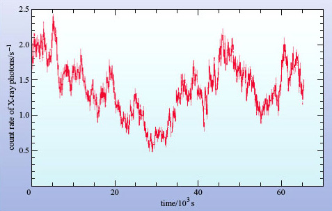
A second approach to estimating the size of an AGN comes from their variability. The continuous spectra of most AGNs vary appreciably in brightness over a one-year timescale, and several vary over timescales as short as a few hours (about 104 s), especially at X-ray wavelengths (see Figure 27). This variability places a much tighter constraint on the size, as you will see.
To take an analogy, suppose you have a spherical paper lampshade surrounding an electric light bulb. When the lamp is turned on, the light from the bulb will travel at a speed c and will reach all parts of the lampshade at the same time, causing all parts to brighten simultaneously. To our eyes the lampshade appears to light up instantaneously, but that is only because the lampshade is so small. In fact, light arrives at your eyes from the nearest point of the lampshade a fraction of a second before it arrives from the furthest visible point (Figure 28).
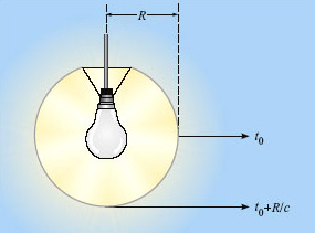
The time delay for the brightening, Δt, is given by

where R is the radius of the lampshade.
Now imagine the shade to be much larger, perhaps the size of the Earth's orbit around the Sun, and the observer is far enough out in space that the shade appears as a point source of light.
What is Δt for a lampshade with the same radius as the Earth's orbit?
Δt = (1.5 × 10¹¹ m)/(3 × 108 m s−1) = 500 s
So even if the lamp is switched on instantaneously, the observer will see the source take about eight minutes to brighten. Now suppose the bulb starts to flicker several times a second. What will an observer see? Even though the lampshade will flicker at the same rate as the bulb, it's clear that the flickering will have no effect on the observed brightness of the lampshade, since each flicker will take 500 seconds to spread across the lampshade and the flickers will be smeared out and mixed together. There is a limit to the rate at which a source (in this case the lampshade) can be seen to change in brightness and that limit is set by its size.
This argument may be inverted to state that if the observer sees a significant change in brightness of an unresolved source in a time Δt, then the radius of the source can be no larger than R = cΔt.
This kind of argument applies for any three-dimensional configuration where changes in brightness occur across a light-emitting surface. Of course, the argument is only approximate - real sources of radiation are unlikely to be perfectly represented by the idealised lampshade model that we have used here. The relationship between the maximum extent (R) of any source of radiation and its timescale for variability (Δt) is usually expressed as

(Where the symbol '∼' is used to imply that the relationship is correct to within a factor of about ten.)
Returning now to the AGN, let us calculate the value of R for an AGN such as MCG-6-30-15. The timescale for variability that we shall use is the shortest time taken for the intensity of the source to double. By inspecting Figure 27 it can be seen that this timescale is about 104 s.
We have R ∼ cΔt, so with Δt = 1 × 10⁴ s, we obtain R ∼ 3 × 10¹² m = 1 × 10⁻⁴ pc. This is a staggeringly small result - it is ten thousand times smaller than the upper limit we calculated from the size of AGN images - and corresponds to about 20 times the distance from the Sun to the Earth. The AGN would easily fit within our Solar System. The argument does not depend on the distance of the AGN. Hence the observed variability of AGNs places the strongest constraint on their size.
One note of caution: the variability of AGNs usually depends on the wavelength at which they are observed. Variations in X-rays, for example, tend to be faster than variations in infrared light. Does this imply that the size of an AGN depends on the wavelength? In a sense, yes, as we are seeing different radiation from different parts of the object. The X-rays seem to come from a much smaller region of the AGN than the infrared emission, so we must be careful when talking about 'the size' of an AGN.
Question 7
An AGN at 50 Mpc appears smaller than 0.1 arcsec in an optical observation made by the Hubble Space Telescope, and shows variability on a timescale of one week. Calculate the upper limit placed on its size by (a) the angular diameter observation, and (b) the variability observation.
Answer
(a) An angular size limit of 0.1 arcsec corresponds to an angle in radians of

Multiplying this by the distance shows that the upper limit on the size is

(b) A week is 7 days which is 7 × 24 × 60 × 60 s. The upper limit from the variability is

(Thus variability constraints provide a much lower value for the upper limit to the size of the AGN than does the optical imaging observation.)
Other evidence also indicates the small size of AGNs. Radio astronomers operate radio telescopes with dishes placed on different continents. This technique of very long baseline interferometry (VLBI) is able to resolve angular sizes one hundred or so times smaller than optical telescopes can. Even so, AGNs remain unresolved.
4.3 The luminosity of AGNs
It is instructive to express the luminosity of an AGN in terms of the luminosity of a galaxy like our own. The figure may then be converted into solar luminosities, if we adopt the figure of 2 × 10¹⁰L⨀ for the luminosity of our Galaxy.
Consider a Seyfert galaxy first. At optical wavelengths the point-like AGN is about as bright as the remainder of the galaxy, which radiates mainly at optical wavelengths. But the AGN also emits brightly in the ultraviolet and the infrared, radiating at least three times its optical luminosity. So one concludes that for a typical Seyfert, the AGN has at least four times the luminosity of the rest of the galaxy.
We have seen that a characteristic of a quasar is that its luminous output is dominated by emission from its AGN. However quasar host galaxies are not less luminous than normal galaxies, so the AGNs of quasars must be far brighter than normal galaxies and must also be considerably more luminous than the AGNs of Seyfert galaxies.
In the case of a radio galaxy, the AGN may not emit as much energy in the optical as Seyfert and quasar AGNs, but an analysis of the mechanism by which the lobes shine shows that the power input into the lobes must exceed the luminosity of a normal galaxy by a large factor, and the AGN at the centre is the only plausible candidate for the source of all this energy.
A similar conclusion for AGN luminosity follows for blazars, which appear to be even more luminous than quasars. We examine why in Section 4.7.
Question 8
Calculate the luminosity of an AGN that is at a distance of 200 Mpc, and appears as bright in the optical as a galaxy like our own at a distance of 100 Mpc. Assume that one-fifth of the energy from the AGN is at optical wavelengths.
Answer
The relationship between flux density F, luminosity L and distance d can be given by the following equation:

Using this relationship it can be seen that if the AGN is at twice the distance but appears as bright as the normal galaxy in the optical, then it must be emitting four times the optical light of the normal galaxy like our own. If only one-fifth of the AGN's energy is emitted in the optical, then its luminosity is 4 × 5 = 20 times that of the normal galaxy like our own, assuming that (as usual) the normal galaxy emits mostly at optical wavelengths. The AGN luminosity is thus about 20 × 2 × 1010L⊙ = 4 × 10¹¹L⊙.
One can conclude that AGNs in general have luminosities of more than 2 × 10¹⁰L⊙ produced within a tiny volume. Stop to ponder this statement for a minute. The power output of the Sun is so large that it is hard to comprehend; the number 2 × 10¹⁰ is even more difficult to imagine! Putting together over 2 × 10¹⁰ Suns' worth of luminosity inside an AGN is well beyond the powers of imagination of most of us. One Sun's worth of luminosity is about 4 × 1026 W, so a typical AGN has a luminosity of more than 8 × 1036 W. In fact, that's quite modest for an active galaxy, so for the purposes of this course we shall adopt a more representative value of 1038 W as the characteristic luminosity of an AGN.
You are now in a position to appreciate the basic problem in accounting for an AGN. It produces an enormous amount of power (luminosity) in what is astronomically speaking a tiny volume. This source of power is known as the engine. Current ideas about the workings of this engine are discussed in the next section.
4.4 A supermassive black hole
A black hole is a body so massive and so small that even electromagnetic radiation, such as visible light, cannot escape from it. It is its combination of small size and very strong gravitational field that makes it attractive as a key component of the engine that powers an AGN. There is good evidence of a black hole of mass 2.6 × 10⁶M⊙ at the centre of the Milky Way. As you will see, it turns out that much more massive black holes are needed to explain AGNs, and these are referred to as supermassive black holes.
A black hole, supermassive or otherwise, is such a bizarre concept that it is worth recapping. The material of which it is made is contained in a radius so small that the gravity at its 'surface', the so-called event horizon, causes the escape speed to exceed the speed of light. According to classical physics, any object that falls into it can never get out again. Even electromagnetic radiation cannot escape, which is why the hole is called 'black'. What goes on inside the black hole is academic - no one can see. What might be seen is activity just outside the event horizon where the gravitational field is strong, but not so strong as to prevent the escape of electromagnetic radiation. It is this surrounding region that is of most interest to astronomers.
The radius of the event horizon is called the Schwarzschild radius and is the distance at which the escape speed is just equal to the speed of light. It is given by

Let us now calculate the maximum mass M of a black hole that is small enough to fit inside an AGN. In Section 4.2 you found that an AGN that varies on a timescale of one day must have a radius less than 3 × 10¹² m. We shall see later that all of the emission from the AGN must come from a region that is outside of the Schwarzschild radius and that the size of this emission region is a few times bigger than RS. Consequently, for this approximate calculation we shall adopt a size for RS that is a factor of ten smaller than the size we calculated above for the emission region, i.e. RS = 3 × 10¹¹ m. Then, from Equation 3.4,
which is equivalent to

This result shows that is clearly possible to fit a black hole with an enormous mass within an AGN, although it does not prove that the central black hole has to be this massive. We will shortly see that there is a different argument that does show that mass of any black hole at the centre of an AGN must be about 108M⊙. This is usually adopted as the 'standard' black hole mass in an AGN. It is some 107 times greater than the masses of the black holes inferred to exist in some binary stars that emit X-rays. Hence, the name supermassive black hole has been adopted.
4.5 An accretion disc
What will happen to matter that comes near a black hole? Consider a gas cloud moving to one side of the black hole, such as cloud A in Figure 29.
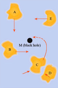
The hole's gravity will accelerate the gas cloud towards it. The cloud will reach its maximum speed when it is at its closest approach to the black hole, but will slow down again as it moves away; it will then move away to a distance at least as great as the distance from which it started. Thus far nothing is new; the gas cloud will behave exactly as it would if it came near some other gravitationally attracting object, such as a Sun-like star.
Now, let us extend the argument to a number of gas clouds being accelerated towards the black hole from different directions in space. This time, as the gas clouds get to their closest approach they will collide with each other, thus losing some of the kinetic energy they had gained as they fell towards the hole. Therefore some, but not all, of the clouds of gas will have slowed to a speed at which they cannot retreat, so they will go into an orbit around the hole. Further collisions amongst the gas clouds will tend to make their orbits circular, and the direction of rotation will be decided by the initial rotation direction of the majority of the gas clouds. The effect of the collisions will be to heat up the gas clouds; the kinetic energy they have lost will have been converted into thermal energy within each cloud, and so the cloud temperature will rise.
So far, we can envisage a group of warm gas clouds in a circular orbit about the black hole. But the clouds of gas are of a finite size and, because they move in a Keplerian orbit, the inner parts of the gas clouds will orbit faster than the outer parts. A form of friction (viscosity) will act between neighbouring clouds at different radii and they will lose energy in the form of heat. The consequence of this is that the inner parts of the gas clouds will fall inwards to even smaller orbits. This process will continue until a complete accretion disc is formed around the black hole (Figure 30).
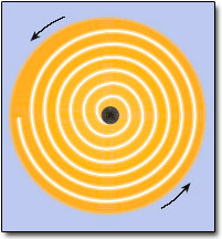
The accretion disc acts to remove angular momentum from most of the gas in the disc so that if you look at the path of a small part of one gas cloud, you can see that it will spiral inwards. Since angular momentum is a conserved quantity the accretion disc does not actually diminish the total angular momentum of the system - it simply redistributes it such that most gas in the disc will move inwards. This process occurs only for a viscous gas - planets in the Solar System do not show any tendency to spiral in to the Sun because interplanetary gas is very sparse. The viscosity causes the gas to heat up further, the thermal energy coming from the gravitational energy that was converted into kinetic energy as the gas fell towards the hole. The heating effect will be large for objects with a large gravitational field and so we might expect that accretion discs around black holes will reach high temperatures and become luminous sources of electromagnetic radiation.
The gradual spiralling-in of gas through the accretion disc comes to an abrupt end at a distance of a few (up to about five) Schwarzschild radii from the centre of the black hole. At this point the infalling material begins to fall rapidly and quickly passes through the Schwarzschild radius and into the black hole. Note that the accretion disc is located outside the event horizon, where the heat can be radiated away as electromagnetic radiation. The accretion model is of such interest because an accretion disc around a massive black hole can radiate away a vast amount of energy, very much more than a star or a cluster of stars. It is this radiated energy that is believed to constitute the power of an AGN.
You may be wondering how large the accretion disc is; after all, the accretion disc as well as the black hole has to fit inside the AGN. The accretion disc gets hotter and therefore brighter towards its inner edge. The brightest, and hence innermost part is what matters. Since this is at only a few times the Schwarzschild radius, there is no problem of size.
Estimate the extent of the brightest part of the accretion disc for a black hole of mass 108M⊙. How does this compare with the radii of planetary orbits in the Solar System?
From Section 4.4 we know that the Schwarzschild radius is about 3 × 10¹¹ m, which is twice the radius of the Earth's orbit or 2 AU. The brightest part of the accretion disc could then extend to about five times this distance or about 10 AU, which is about the radius of Saturn's orbit.
4.6 Accretion power
Calculations based on the above accretion disc hypothesis show that if a mass m falls into the black hole, then the amount of energy it can radiate before it finally disappears is about 0.1 mc2, or about 10% of its rest energy. Other than matter-antimatter annihilation, this is the most efficient process for converting mass into energy ever conceived. A comparable figure for the nuclear fusion of hydrogen in stars is only 0.7% of the rest energy of the four hydrogen nuclei that form the helium nucleus.
Question 9
How much energy could be obtained from 1 kg of hydrogen (a) if it were to undergo nuclear fusion in the interior of a star, (b) if it were to spiral into a black hole? Would you expect to get more energy if it were to chemically burn in an oxygen atmosphere?
Answer
A mass m has a rest energy of mc2.
(a) If 1 kg of hydrogen were to undergo nuclear fusion to produce helium, the energy liberated would be 0.007 (i.e. 0.7%) of its rest energy:

(b) If 1 kg of hydrogen were to fall into a black hole, the energy liberated would be approximately
0.1mc2 = 0.1 × 1 × (3 × 108ms−1)2 J = 9 × 10¹⁵ J.
You would expect much less energy from the chemical reaction.
Now let us apply the idea of an accreting massive black hole to explain the luminosity of an AGN. We have to explain an object of small size and large luminosity. The Schwarzschild radius of a black hole is very small, and the part of the accretion disc that radiates most of the energy will be only a few times this size. The luminosity will depend on the rate at which matter falls in. Suppose that the matter is falling in at the rate Q (with units of kg s−1), this is known as the mass accretion rate. We can now work out the value of Q to produce a luminosity L by writing

Using the values L = 1038 W and c = 3 × 10⁸ m s−1, we get Q = 1022 kg s−1. Converting this into solar masses per year using 1M⊙ ≈ 2 × 1030 kg and 1 year ≈ 3 × 10⁷ s, we get Q ≈ 0.2M⊙ per year. Is there a large enough supply of matter for a fraction of a solar mass to be accreted every year? Most astronomers think that the answer is yes, and that even higher accretion rates are plausible - after all our own Galaxy has 10% of its baryonic mass in gaseous form, so there is at least 1010M⊙ of gas available.
Does this estimate of the accretion rate require a supermassive black hole, or will any black hole such as one of 5M⊙ do?
The mass of the black hole does not enter into the above calculation. So on this basis a 5M⊙ black hole would seem to be sufficient.
Moreover, the mass calculated in Section 4.4 is an upper limit. So, why is a supermassive black hole needed? To see why, we ask: is there any limit to the power L that can be radiated by an accretion disc around a black hole, or can one conceive of an ever-increasing value of L if there is enough matter to increase Q?
There is a limit to the amount of power that can be produced, and it is called the Eddington limit. As the black hole accretes faster and faster, the luminosity L will go up in proportion, that is to say the accretion disc will get brighter and hotter. Light and other forms of electromagnetic radiation exert a pressure, called radiation pressure, on any material they encounter. (This pressure is difficult to observe on Earth because it is difficult to find a bright enough light source.)
Around an accreting black hole with a luminosity of 1038 W, the radiation will be so intense that it will exert a large outward pressure on the infalling material. If the force on the gas due to radiation pressure exactly counteracts the gravitational force, accretion will cease. This process acts to regulate the luminosity of an accreting black hole.
To work out the Eddington limit, it is necessary to balance radiation pressure against the effects of the black hole's gravity. Consider an atom of gas near the outer edge of the accretion disc. The force on it due to radiation pressure is proportional to L, whereas the gravitational force is proportional to the mass M of the black hole (assuming the mass of the accretion disc to be negligible). A balance is achieved when LE = constant × M, where LE is the Eddington limit. Full calculations give

This is the upper limit of the luminosity of a black hole of mass M - the luminosity can be lower than LE but not higher. The larger the mass M, the greater the value of LE.
In fact, this is only a rough estimate. It assumes that the accreting material is ionized hydrogen (a good assumption) and that the hole is accreting uniformly from all directions (which is not a good assumption). The Eddington luminosity may be exceeded, for example, if accretion occurs primarily from one direction and the resulting radiation emerges in a different direction. Nonetheless, it is a useful approximation.
Putting L = 1038 W into Equation 3.6, we find that M= 7.7 × 10⁶M⊙. So we see that we do need a supermassive black hole to account for the engine in an AGN, and 108M⊙ is usually assumed.
In summary, then, the Eddington limit means that the observed luminosity of quasars requires an accreting supermassive black hole with a mass of order 108M⊙; the accretion rate is at least a significant fraction of a solar mass per year; and the Schwarzschild radius is about 3 × 10¹¹ m.
4.7 Jets
You have seen that two kinds of active galaxies - quasars and radio galaxies - are often seen to possess narrow features called jets projecting up to several hundred kiloparsecs from their nuclei. If these are indeed streams of energetic particles flowing from the central engine, how do they fit with the accretion disc model? How could the jets be produced?
The answers to these questions are not fully resolved, but there are some aspects of the model of the central engine which probably play an important part in jet formation. A key idea is that the jets are probably aligned with the axis of rotation of the disc - since this is the only natural straight-line direction that is defined by the system. This much is accepted by most astrophysicists, but the question of how material that is initially spiralling in comes to be ejected along the rotation axis of the disc at relativistic speeds (i.e. speeds that are very close to the speed of light) is an unsolved problem.
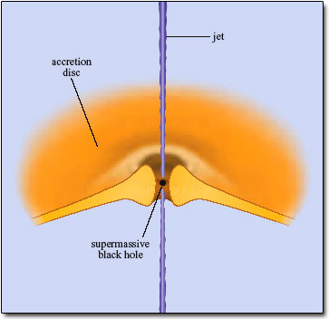
One mechanism that has been suggested requires that at distances very close to the black hole the accretion disc becomes thickened and forms a pair of opposed funnels aligned with the rotation axis, as illustrated in Figure 31. Within these funnels the intense radiation pressure causes the acceleration and ejection of matter along the rotation axis of the disc. Unfortunately, this model fails in that it cannot produce beams of ejected particles that are energetic enough to explain the observed properties of real jets. Other variants of this scenario, and in particular those in which the magnetic field of the disc plays a major role in the ejection of jets are under investigation but do not yet offer a full explanation of the jet phenomenon.
If jets are ejected along the rotation axis of the disc, then why do quasars and the more powerful radio galaxies generally only appear to have a single jet? It seems improbable that the engine produces a jet on one side only, and it is thought that there are indeed two jets but only one is visible. In this model, two jets are emitted at highly relativistic speeds, and one of them is pointing in our direction and the other is pointing away. Due to an effect called relativistic beaming, the radiation from the jets is concentrated in the forward direction. The jet consequence of this is that if a jet is pointing even only very approximately towards us it will appear very much brighter than would a similar jet that is pointing in the opposite direction. (The special case of what happens when a jet is pointing directly at us will be considered in the next section.)
Question 10
Estimate the accretion rate on to a black hole needed to account for the luminosity of a Seyfert nucleus that has twice the luminosity of our Galaxy. Express your answer in solar masses per year. What, other than the mass accretion rate, limits the luminosity?
Answer
For the Seyfert nucleus, L = 4 × 10¹⁰L⊙ = 1.6 × 1037 W. By Equation 3.5, Q = L(0.1c2). Substituting for L,
This can be converted into solar masses per year, by using 1 year ≈ 3 × 10⁷ s, and M⊙ ≈ 2 × 1030 kg, giving
The Eddington limit places an upper limit on the luminosity for a black hole of given mass.
5 Models of active galaxies
5.1 Introduction
So far we have seen how the properties of the central engine of the AGN can be accounted for by an accreting supermassive black hole. Though there are many questions still to be resolved, this model does seem to be the best available explanation of what is going on in the heart of an AGN. But of course all AGNs are not the same. We have identified four main classes and in this section we will attempt to construct models that reproduce the distinguishing features of these four classes.
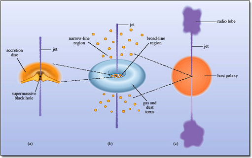
Figure 32 shows the basic model that has been proposed for AGNs. It is a very simple model, and does not account for all AGN phenomena, but it does give you a flavour of the kinds of ideas that astrophysicists are working with. You can see that the central engine (the supermassive black hole and its accretion disc) is surrounded by a cloud of gas and dust in the shape of a torus (a doughnut shape). The gap in the middle of the torus is occupied by clouds forming the broad-line region and both in turn are enveloped by clouds forming the narrow-line region.
We begin by looking at the torus.
5.2 The obscuring torus
If an AGN consisted solely of the central engine, observers would see X-rays and ultraviolet radiation from the hot accretion disc (accounting for the 'the big blue bump' in Figure 17) and, apart from the jets, very little else. To account for the strong infrared emission from many AGNs, the model includes a torus of gas and dust that surrounds the central engine.
The dust particles - which are usually assumed to be grains of graphite - will be heated by the radiation from the engine until they are warm enough to radiate energy at the same rate at which they it receive it. As dust will vaporise (or sublimate) at temperatures above 2000 K, the cloud must be cooler than this.
Question 11
Assuming that dust grains radiate as black bodies, estimate the range of wavelengths that will be emitted from the torus.
Note: A black-body source at a temperature T has a characteristic spectrum in which the maximum value of spectral flux density (Fλ) occurs at a wavelength given by Wien's displacement law
Answer
Wien's displacement law relates the temperature of a black body to the wavelength at which the spectral flux density has its maximum value. In this case, the dust grains on the inner edge of the torus will be at 2000 K, so their peak emission will be at
So, λmax is about 1.5 μm.
Grains further from the engine will be cooler, and their emission will peak at longer wavelengths, so the torus can be expected to radiate in the infrared at wavelengths of 1.5 μm or longer. (Note that although the spectrum emitted by dust grains is not a black-body spectrum, it is similar enough for the above argument to remain valid.)
So such a dust cloud will act to convert ultraviolet and X-ray emission from the engine into infrared radiation, with the shortest wavelengths coming from the hottest, inner parts of the cloud.
From a very simple dust cloud model, it is easy to understand why AGNs so often emit most of their radiation in the infrared. Almost certainly, dust heated by the engine is observed in most AGNs, although the dust may be more irregularly distributed than in our simple model, and the torus may have gaps in it. Some small amount of the infrared radiation will generally come from the engine itself, though, and in BL Lacs it is probable that most of the infrared radiation comes from the engine. The variability that was discussed in Section 4.2 applies to radiation from the engine at X-ray and optical wavelengths (and sometimes at radio wavelengths). The infrared emission from the torus is thought to vary much more slowly, as you would expect from the greater extent of the torus.
Note that this torus is not the same as the accretion disc surrounding the black hole, though it may well lie in the same plane and consist of material being drawn towards the engine.
It is possible, using a simple physical argument, to make a rough estimate of the inner radius of the torus by asking how far from the central engine the temperature will have fallen to 2000 K, the maximum temperature at which graphite grains can survive before being vaporised.
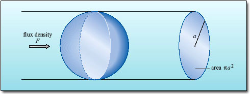
If the engine has a luminosity, L, then the flux density at a radius r from the engine will be L/4![]() r2. A dust grain of radius a will intercept the radiation over an area
r2. A dust grain of radius a will intercept the radiation over an area ![]() a2 (Figure 33) and, if no energy is reflected, the power absorbed will be
a2 (Figure 33) and, if no energy is reflected, the power absorbed will be
The temperature of the dust grain will rise until the power emitted by thermal radiation is equal to the power absorbed. If the grain behaves as a black body we can write
where σ is the Stefan-Boltzmann constant (σ = 5.67 × 10⁻⁸ W m2 K−4).
Here we assume that the temperature of the grain is the same over its whole surface, which would be appropriate if, for instance, the grain were rotating. Next, we make the power absorbed equal to the power radiated
Finally, if we divide both sides by a2, the radius a is cancelled out (as it should - the size of the dust grain should not come into it) and we can rearrange for r to get:
This distance is called the sublimation radius for the dust.
Question 12
Calculate the dust sublimation radius, in metres and parsecs, for an AGN of luminosity 1038 W. (Assume that dust cannot exist above a temperature of 2000 K.)
Answer
From Equation 3.7 we have
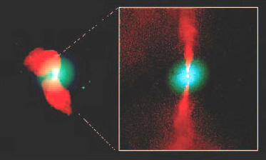
Thus, according to this calculation, the radius of the inner edge of the dust torus is 1.5 × 10¹⁵ m or 0.05 pc. (A more rigorous calculation, which takes account of the efficiency of graphite grains in absorbing and emitting radiation, gives a radius of 0.2 pc.)
For typical luminosities, the inner edge of the torus is three or four orders of magnitude (i.e. 1000 to 10 000 times) bigger than the emitting part of the accretion disc which is contained within the central engine in Figure 31. Even so, the torus cannot be resolved even in high-resolution images. However there is evidence in several galaxies of a much more extensive disc of gas and dust that encircles the AGN. It has been suggested, although not proven, that these discs provide a supply of material that can spiral down into the central regions of the active galaxy - passing into the torus, through the accretion disc, and eventually falling into the black hole itself.One example of such a disc is found in the radio galaxy NGC 4261 which is shown in Figure 34.
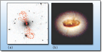
On the left (Figure 34a) you can see a radio image of the jets, superimposed on an optical image of the host galaxy. The highly magnified image (Figure 34b), taken with the Hubble Space Telescope, shows a dark obscuring disc silhouetted against the stellar core of the elliptical host galaxy. This disc is about 250 pc across and very much bigger than the sub-parsec structures that make up the AGN itself. Note that its plane is perpendicular to the axis of the radio jets shown on the left of the figure. Thus the jets seem to be aligned along the rotation axis of the disc, and this lends support to the ideas of jet formation that were outlined in Section 4.7.
5.3 The broad- and narrow-line regions
In our model, the engine is surrounded by gas clouds (Figure 32). You have already seen how common these are in our own and other galaxies, so it is reasonable to expect them to be present in at least the spiral galaxies that contain AGNs. If these gas clouds are illuminated by ultraviolet or X-rays from the engine they will absorb the ultraviolet or X-ray energy, and will emit the characteristic lines of the gases making up the clouds. The most abundant gas in galactic clouds is hydrogen, and, sure enough, the H![]() and other lines of hydrogen appear strongly in the observed spectra of AGNs.
and other lines of hydrogen appear strongly in the observed spectra of AGNs.
What about other spectral lines that might be expected? Fortunately we get clues from objects in our own Galaxy, the HII regions, which consist of gas clouds illuminated by sources of ultraviolet radiation, albeit at a lower luminosity. These HII regions emit strong lines of nitrogen and oxygen, [NII] and [OIII], in the optical. Sure enough, the lines that appear in the optical spectra of AGNs turn out to be just what you would expect from a gas of normal cosmic composition surrounding an AGN.
As you have discovered, there appear to be two kinds of line-emitting regions known as the broad-line region (BLR) and narrow-line region (NLR). If we interpret the spectra in terms of the density (inferred from the presence or absence of forbidden lines) and motion of gas clouds (inferred from line widths), then the BLR corresponds to dense fast-moving clouds and the NLR to low-density, more slowly moving clouds.
It is not possible to see the motion in great detail, but these motions are probably associated with the strong gravitational field surrounding an AGN. The orbital speed of a cloud will increase as the distance from the central black hole decreases. Thus the faster moving BLR clouds are assumed to be closer to the centre than the slower moving NLR clouds.
Broad-line region
In the model, the clouds of the broad-line region surround the central engine within the opening in the middle of the dust torus. The radius of the BLR is of the order of 1014 m, placing it well inside the torus. At this distance from the black hole orbital speeds are several thousand kilometres per second, which is consistent with the typical speed of 5000 km s−1 that is measured from Doppler broadening. The clouds are fully exposed to the intense radiation from the engine (remember that any dust will have vaporised in this region) and will be heated to a high temperature. It is difficult to measure the temperature of BLR clouds, but it appears to be of the order of 104 K.
It has been estimated that the BLR of a typical AGN will have about 1010 clouds covering about 10% of the sky as seen from the central engine. The total mass of gas is less than 10M⊙, so it is utterly negligible compared with the black hole itself.
Broad lines are not seen in every AGN. The general belief among astronomers is that every AGN has a broad-line region, but in some cases our view of the BLR clouds is obscured by the dust torus, so broad lines do not appear in the spectrum.
Narrow-line region
The model places the narrow-line region much further out from the central engine where orbital speeds are lower; 200-900 km s−1 is typical for the NLR.
An important consequence of the NLR being outside the dust torus is that it is always in view, so narrow lines will be seen even if the broad-line emitting gas is obscured.
Question 13
The narrow-line region is the most extensive part of the AGN and envelops all the other components. Like the other parts, it is illuminated by the central engine. Bearing in mind the geometry of the dust torus, describe what the NLR might look like if a spaceship could get close enough to see it. From which direction would the observers have the best view?
Answer
The NLR is illuminated by radiation from the central engine. As the engine is partly hidden by the dust torus, radiation can only reach the NLR through the openings along the axis of the torus. Any gas near the plane of the torus lies in its shadow and will not be illuminated. The visible NLR would take the form of a double cone of light corresponding to the conical beams of radiation emerging from either side of the torus.
The best view would be from near the plane of the torus, where a wedge-shaped glow would be visible on either side of the dark torus.
So the model predicts that the NLR, if we could see it, would have a distinctive shape. You might think that such observations would be impossible, considering the tiny size of an AGN. But the NLR is the outer part of the AGN and has no real boundary. In fact, several NLRs have been imaged by the Hubble Space Telescope and one example, for the Seyfert galaxy NGC 5252, is shown in Figure 35.
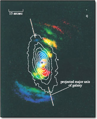
The double wedge shape reveals where the gas is illuminated by radiation shining from the centre of the torus. In this case the emission extends several kiloparsecs from the AGN and is known as an extended narrow-line region. The extended region is simply interstellar gas ionised by the radiation from the engine. This observation, and others like it, provides supporting evidence for the geometry of the dust torus and the NLR.
So even if we cannot observe the inner structure of an AGN, the regions around the nucleus are tantalisingly consistent with the model.
5.4 Unified models
You are now familiar with the main components for building models of AGNs: a central engine powered by an accreting supermassive black hole (with or without jets), clouds of dust, clouds of gas and accretion processes that can organise the gas and dust into a torus-shaped structure. Many attempts have been made to use these components to explain the different types of AGN. Two basic ideas - or perhaps hopes - underlie these models.
First, all AGNs are essentially the same and differ chiefly in the luminosity of the central engine which in turn depends on the mass of the black hole and the mass accretion rate.
Second, if the AGN contains a dust torus then the radiation observed will depend on the direction from which the AGN is viewed. Two possible schemes for such unified AGN models are shown in Figure 36. One is for radio-quiet AGNs and the other is for radio-loud AGNs.
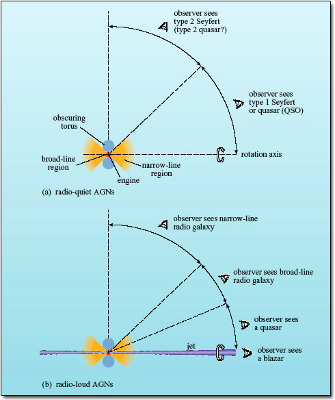
Radio-quiet AGNs
There has been a great deal of debate about whether there really are two different types of Seyfert or whether they can both be accounted for by the same model.
For example, suppose that you look at the model AGN in Figure 36a from a direction not too far from the rotation axis of the torus. You will see X-ray, UV (the 'big blue bump') and other radiation from the engine, broad lines from the broad-line region, narrow lines from the narrow-line region and infrared from the dust torus. You will observe the features associated with a type 1 Seyfert.
If you look at the same model from a direction nearer to the plane of the torus, the X-rays and the broad optical emission lines will be hidden by the torus, and you will observe the features associated with a type 2 Seyfert. Observations strongly suggest that at least some type 2 Seyferts are essentially type 1 Seyferts seen from a different angle. This also accounts for the intermediate types, where the broad-line region is only partly in view.
The galaxy in Figure 35 is described as a type 2 Seyfert. Is this significant?
Yes. In the unified model, type 2 Seyferts are seen from an angle close to the plane of the torus. This is the best viewing angle to see the shape of the NLR, as discussed in Question 13.
Does the same apply to other types of AGN? Radio-quiet quasars (QSOs) appear in many respects to be similar to type 1 Seyferts, showing both broad and narrow emission lines, but are much more luminous. There seems little doubt that Seyferts and radio-quiet quasars differ primarily in luminosity.
Much less is known about 'type 2' quasars without broad lines, analogous to the type 2 Seyferts. It may be that the dust torus around the more luminous quasars is diminished by the intense radiation, hence revealing the BLR from a large fraction of all possible orientations. On the other hand, some astronomers speculate that a recently discovered class of highly luminous galaxies that emit strongly in the far infrared may be the missing type 2 quasars concealed behind their dust clouds.
Radio-loud AGNs
The second model (Figure 36b) is similar to the first, but now the engine is producing a pair of jets that will eventually end in a pair of lobes, as seen in radio galaxies and some quasars.
Looking at the model from the side, one expects to see narrow lines in the spectrum (but not broad lines) and two jets surrounded by extended lobes. This is a narrow-line radio galaxy. At an angle closer to the jet axis the broad-line region comes into view and a broad-line radio galaxy is seen. So far this is analogous to the two types of Seyfert, but now another effect comes into play. As you saw in Section 4.7, relativistic beaming will cause an approaching jet to be brighter than a receding jet, so as the angle decreases one jet will fade at the expense of the other and a radio galaxy with a single jet will now be visible (though there may well be two lobes).
As the angle continues to decrease the intense source of radiation surrounding the black hole comes into view and the object appears as a quasar, with never more than one visible jet. Finally, a blazar is seen when the torus is face-on to the observer who is looking straight down the jet. One distinguishing feature of the blazars is that the spectrum is dominated by a smooth continuous spectrum which is what one would expect if the radiation is coming from the jet itself. Another feature of blazars is their rapid variability over a wide range of wavelengths, and this again is to consistent with the idea of the emission arising from a jet. BL Lacs would correspond to the less powerful radio galaxies and OVVs to the more powerful ones.
Unification of the radio-loud sources is more contentious and this model is by no means the last word on the subject. It has been difficult to reconcile all the observed properties of the AGNs with the model. For example, one test would be to examine whether the numbers of different kinds of AGN are consistent with what the model predicts.
Suppose that radio galaxies, radio-loud quasars and blazars were all the same kind of object but seen from different angles. From Figure 36b, which would you expect to be the most common? Which the least common?
Radio galaxies would be seen over the widest range of angles, so these would be the most common. Blazars, on the other hand, would only be seen over a narrow range of angles and would be relatively rare.
This simple approach is complicated by two things. First, AGNs vary greatly in luminosity and distance, so the number observed is not necessarily a measure of how common they are. Powerful or nearby objects are more likely to show up in a survey than weak or distant objects. Second, AGNs are visible over such large distances that the light from the more remote ones started on its journey when the Universe was considerably younger than it is today. The most distant quasars may no longer exist in the form in which they are observed. We shall return to that idea shortly.
At the moment the jury is still out, as they say, but astronomers are confident that even if the different kinds of radio-loud AGNs are not identical siblings, they are at least close cousins.
Perhaps the most difficult question is why some AGNs are radio-loud while most are radio-quiet. You have seen that the radio-quiet AGNs appear to reside in spiral galaxies while the radio-loud AGNs are in ellipticals. It was once thought that the presence of gas in spiral galaxies acted to suppress the emergence of jets from the engine, but that idea is no longer favoured. Current thinking relates the presence of jets to the angular momentum of the black hole, with only the faster-spinning black holes able to produce jets. The novel element is that a high spin rate could be achieved not by accretion but by the merger of two massive black holes following the collision and merger of their host galaxies. There is other evidence that giant elliptical galaxies are formed from mergers, so this seems a plausible, if yet unproven, explanation as to why the radio-loud sources tend to be found in ellipticals.
6 Outstanding Issues
6.1 Introduction
The active galaxy model is very attractive. Indeed, it is so attractive that it is easy to overlook the many problems that remain. We will now consider some of the outstanding questions about the origin and evolution of active galaxies, focusing on two questions: do supermassive black holes really exist? And where are active galaxies now?
6.2 Do supermassive black holes really exist?
One outstanding feature of the black-hole model is that the black hole must be supermassive. Can one at least detect the presence of a massive central object?
How might a massive central object be detected using information from galactic rotation curves?
By measuring rotation speeds near the nucleus of the galaxy. The faster the rotation speeds, the greater the enclosed mass.
So the answer is yes. In NGC 4151, a prominent type 1 Seyfert galaxy, the broad lines are observed to vary as well as the continuous spectrum. The line variations lag about 10 days behind associated variations in the continuous spectrum. The usual interpretation is that the variations commence in the engine, where the continuous spectrum originates, then take 10 days to 'light up' the broad-line region. So the broad-line region must be a distance r of about 10 light-days from the engine. Supposing that the broad lines are Doppler-broadened by rotation around the engine, then one has a picture of regions of gas moving at a speed ν of about 7000 km s−1 around a central engine of mass M at a radius r. The value of M can now be calculated from ν and r. Using the following equation

with r = 10 light-days (3 × 10¹⁴ m), and v = 7 × 10⁶ m s−1, and converting into solar masses, we obtain M = 108M⊙. This is consistent with the value of M for an accreting black hole calculated from consideration of the Eddington limit.
This approach has been very productive. One of the most studied active galaxies is the radio galaxy M87 which you have seen in Figure 24. Since the late 1970s astronomers have suspected it contains a supermassive black hole and the most recent observations with the Hubble Space Telescope reveal a rotating disc of gas only 16 pc from the centre. If the equation above applies, then the mass of the central object is around 3 × 10⁹ M⊙.
In the mid-1990s it became possible to probe even closer to the centre of an AGN. Measurements of rotating gas within 0.18pc of the core of NGC 4258, a weak Seyfert galaxy, showed that an object of around 4 × 10⁷M⊙ must be at the centre. Similar measurements have been made of other active galaxies.
Another intriguing observation comes from the Seyfert galaxy MCG-6-30-15, whose variability was illustrated in Figure 27. Its X-ray spectrum shows an extremely broad emission line, 100 000 km s−1, which is believed to come from the accretion disc itself. The line is greatly distorted as if it originated in the intense gravitational field near a black hole, but it has not yet been possible to derive the mass of the black hole.
You have now heard some of the evidence that accreting massive black holes really do provide the engine power for AGNs. Do you think it is convincing?
If not, the alternatives are not very promising. The only other idea still in the running is a 'nuclear starburst' model, a cluster of young, massive stars with frequent supernova explosions, but this does not fit the observations so well. It remains interesting because of its similarity to the processes occurring in starburst galaxies. If a supermassive black hole is the leading contender, it is because no-one has yet thought of anything better.
Question 14
How convincing is the scientific evidence for: (a) the existence of accreting massive black holes in AGNs; (b) the occurrence of nuclear fusion in the Sun and other stars; (c) the laws governing the orbits of the planets around the Sun?
Answer
(a) An accreting massive black hole is a hypothesis that has been thought up to account for AGNs. There is really no conclusive evidence to support the hypothesis. However, no-one has a better idea of how to produce enough power for an AGN in the small volume.
(b) The occurrence of nuclear fusion in the Sun was originally a hypothesis proposed to explain the Sun's energy source. The whole theory of the structure and evolution of stars of different mass and different composition has been based on the nuclear fusion idea. The agreement of this theory with observations is strong confirmation that the nuclear fusion idea is correct.
(c) The laws governing the motion of the planets round the Sun account for all planetary motions ever observed and allow future motions to be predicted. This is the strongest evidence for their correctness. It could even be said that people have conducted experiments by launching spacecraft that are found to move according to these same laws.
6.3 Where are they now?
At the beginning of this course we asked whether active galaxies really are in a class of their own or whether most galaxies go through an active stage at some point in their lives. We can shed some light on this by looking for evidence that active galaxies evolve.
The first question is where AGNs came from. No-one knows how supermassive black holes formed and the question is intimately tied up with the origins of galaxies which is itself a vigorously debated topic. But it is likely that close interactions and collisions between galaxies were much more common than they are now, and such disturbances played an important part in providing material to feed a growing black hole and to stimulate AGN activity. Even today, active galaxies are more likely than normal galaxies to be within the gravitational influence of a companion galaxy - about 15% of Seyferts have companions compared with 3% of normal galaxies - and you have seen examples such as Centaurus A (see Figure 23) which seem to be the result of a recent merger.
Next we can ask how long AGNs live. As indicated earlier, we observe distant objects not as they are today, but as they were at the time their light was emitted. As electromagnetic radiation takes 3.2 million years to travel one megaparsec, even the relatively nearby quasar, 3C 273, is seen as it was some 2.5 billion years ago, and those with the highest observed redshifts are seen perhaps only a billion years after the beginning of the Universe. So by studying the most remote quasars and comparing them with closer ones, it should be possible to see if they have changed over the lifetime of the Universe.
Astronomers have worked out the numbers of quasars in a given volume of space for different redshifts. When the expansion of the Universe is taken into account, the number density of quasars seems to have reached a maximum around a redshift of 2-3 about 10 billion years ago and has been declining sharply ever since. Indeed, quasars were something like 103 times more common then than they are now. This suggests that the quasar phenomenon is short-lived, by cosmic standards. Where have they all gone?
Bearing in mind what you already know about quasars, what would you expect a 'dead' quasar to look like?
As a quasar is believed to be an AGN within an otherwise normal galaxy, a dead quasar would look like a normal galaxy without an AGN.
How could you tell whether a normal galaxy once had a quasar inside it?
Look in the nucleus! If the black hole model is correct, dead quasars will leave a supermassive black hole behind them.
So if quasars are indeed powered by supermassive black holes, it should be possible to find the 'relic' black holes in our local region of space, even where there are no obvious AGNs. If a galaxy was once a quasar the black hole will still be there; it is, after all, rather difficult to dispose of an object of 108M⊙.
In the last section you learned about the rotation studies used to measure the masses of black holes in AGNs - M87 holds the record at about 3 billion M⊙. The same methods have been used to examine the centres of normal galaxies and one result has been a dark object with a mass of about 2 × 10⁶M⊙ residing at the centre of the Milky Way.
There is even more compelling evidence that M31 (the Andromeda Galaxy), which is the nearest big spiral to the Milky Way, contains an object of 3 × 10⁷M⊙. Even its small elliptical companion, M32, hides an object of 2 × 10⁶M⊙. Several more otherwise normal galaxies, most of them not far from the Milky Way, appear to possess supermassive objects, and the closer the observations get to the centre, the more confident astronomers are that these concentrations of mass are indeed black holes.
The modern view is that many, perhaps most, galaxies contain supermassive black holes, though we know that some do not (another nearby spiral, M33, has been shown to have no supermassive black hole, or at least nothing more massive than 3000M⊙). The ubiquity of supermassive black holes means that it is possible that many of the galaxies that we observe as 'normal' at the present time might have gone through an active stage in the past. It should be stressed however that there is no definite proof that this scenario is correct.
The idea that extinct (or perhaps, dormant) quasars might be lurking quite close to us is intriguing and also, perhaps, alarming. One important question is why the quasars died. It cannot simply be because of a lack of fuel. As you saw earlier, less than one solar mass a year is needed to fuel a typical AGN. This is a relatively small amount and could easily be provided by the host galaxy. However, in order to fall into the central black hole, any surrounding gas clouds must also lose angular momentum. You saw earlier that very close to the black hole, material can only spiral inwards because of the viscosity of the gas in the accretion disc. The mechanism by which more distant orbiting clouds may spiral in towards the centre of an active galaxy is still something of a mystery. However, it seems likely that whatever process operates to cause material to spiral inwards, it will be the clouds that are closest to the AGN that will be most strongly affected. Thus it has been suggested that as time passes the AGN may 'sweep clean' the gas from its immediate environment. If, as is expected, this gas is not replenished from clouds that are on orbits further away from the AGN then the mass accretion rate will drop, and the active galaxy will fade over time.
However this is not the end of the story, since if the central regions of the galaxy are disturbed - perhaps by a galactic collision or merger - then it is possible that the gas supply to the black hole could be temporarily restored and the AGN could then spring back into life. This may be what is currently happening in the case of the Centaurus A (Figure 23), which we have seen is a galaxy that appears to have undergone a recent merger. This scenario seems plausible, but is extraordinarily difficult to test in detail. However if this view of how AGN are fuelled is correct, then it is possible, although perhaps not very likely, that one day the black hole at the centre of the Milky Way could begin to accrete matter and start shining like a quasar.
7 course Summary
7.1 The spectra of galaxies
The spectrum of a galaxy is the composite spectrum of the objects of which it is composed.
The optical spectrum of a normal galaxy contains contributions from stars and HII regions. An elliptical galaxy has no HII regions and has an optical spectrum that looks somewhat like a stellar spectrum but with rather fainter absorption lines. A spiral galaxy has both stars and star-forming regions, and its optical spectrum is the composite of its stars and its HII regions (which show rather weak emission lines).
The widths of spectral lines from a galaxy may be affected by Doppler broadening due either to thermal motion or to bulk motion of the emitting material.
An active galaxy has an optical spectrum that is the composite of the spectrum of a normal galaxy and powerful additional radiation characterised by strong emission lines. The broadening comes from bulk motion of the emitting gas.
A broadband spectrum comprises radiation from a galaxy over all wavelength ranges. To judge a broadband spectrum fairly, it is necessary to use a λFλ plot on logarithmic axes which is called a spectral energy distribution (SED).
The SEDs of normal galaxies peak at optical wavelengths while the SEDs of active galaxies show emission of substantial amounts of energy across a wide range of wavelengths that cannot be attributed to emission from stars alone.
7.2 Types of active galaxy
All active galaxies have a compact, energetic nucleus - an AGN.
Seyfert galaxies are spiral galaxies with bright, point-like nuclei which vary in brightness. They show excesses at far infrared and other wavelengths, and have strong, broad emission lines.
Quasars resemble very distant Seyfert galaxies with very luminous nuclei. They are variable. About 10% are strong radio sources thought to be powered by jets of material moving at speeds close to the speed of light.
Radio galaxies are distinguished by having giant radio lobes fed by one or two jets. They have a compact nucleus like Seyfert galaxies. The compact nucleus is variable, and its emission lines may be broad or narrow.
Blazars exhibit a continuous spectrum across a wide range of wavelengths and emission lines, when present, are broad and weak. They are variable on very rapid timescales.
7.3 The central engine
An object that fluctuates in brightness on a timescale Δt can have a radius no greater than R ∼ cΔt.
The point-like nature of AGNs and their rapid variability imply that the emitting region is smaller than the size of the Solar System.
The central engine of a typical AGN is believed to contain a supermassive black hole of mass ∼108M ⊙ and Schwarzschild radius ∼3 × 10¹¹ m (2 AU).
Infalling material is thought to form an accretion disc around the black hole, converting gravitational energy into thermal energy and radiation. A typical AGN luminosity of 1038 W can be accounted for by an accretion rate of 0.2M⊙ per year.
The maximum luminosity of an accreting black hole is given by the Eddington limit, at which the gravitational force on the infalling material is balanced by the radiation pressure of the emitted radiation.
Jets are thought to be ejected perpendicular to the accretion disc.
7.4 Models of active galaxies
The standard model of an AGN consists of an accreting supermassive black hole (the engine) surrounded by a broad-line region contained within a torus of infrared emitting dust and a narrow-line region.
Unified models attempt to explain the range of AGNs on the assumption that they differ only in luminosity and the angle at which they are viewed.
One type of model attempts to unify radio-quiet AGNs. Type 1 Seyferts and type 2 Seyferts differ only in the angle at which they are viewed. Radio-quiet quasars (QSOs) are similar to Seyferts but much more powerful. Evidence for this model is strong.
Another set of models, in which the engine emits a pair of jets, attempts to unify radio-loud AGNs. The observer sees a radio galaxy, a quasar or a blazar as the viewing angle moves from side-on to the jets to end-on. These models remain controversial and there is not yet a consensus on whether such a unification is possible.
The difference between radio-loud and radio-quiet AGNs may lie in the angular momentum of their black holes. The faster-spinning holes may have arisen from mergers of black holes resulting from the collision of their host galaxies.
7.5 Outstanding issues
Evidence from rotation studies shows that some AGNs do indeed contain compact, supermassive objects within them, though there is no direct evidence that these are black holes.
Quasars were most abundant at redshifts of 2-3 and have been declining in number for the last 10 billion years.
It seems probable that AGNs fade with time as the supply of accreting material is used up. There is speculation that AGNs may be rejuvenated as a result of galactic collisions or mergers.
Supermassive black holes found in the nuclei of the Milky Way and other galaxies may be the remnants of extinct AGNs.
7.6 Questions
Question 15
Suppose that a galaxy has emission lines in its optical spectrum. A line of wavelength 654.3 nm is broadened by 2.0 nm. Estimate the velocity dispersion of the gas giving rise to the broadened spectral line. Is it likely to be a normal galaxy?
Answer
For the gas motion use Equation 3.1, Δλ/λ = Δv/c, where Δv is the velocity dispersion. Then Δλ/λ = 2.0 nm/654.3 nm ≈ 0.0030.
Thus the overall spread of internal speeds is Δv ≈ 0.0030 × c ≈ 900 km s−1, which is too large for a normal galaxy.
Question 16
Calculate λFλ flux densities in W m−2 in the radio, the far infrared and the X-ray regions, given the Fλ and λ values listed in Table 2. Which wavelength region dominates?
| Region | λ | Fλ/W m−2 μm−1 | λFλ/W m−2 |
|---|---|---|---|
| Radio | 10 cm | 10−28 | |
| far-IR | 100 μm | 10−23 | |
| X-ray | 10−10 m | 10−20 |
Answer
In the radio wave region, λ = 105 μm so

In the far infrared region λ = 100 μm so that

In the X-ray region, λ = 10−4 μm so

The largest of these λFλ values is 10−21 W m−2, so we conclude that the far-infrared emission dominates.
Question 17
Suppose that an unusual galaxy has broadband spectral flux densities Fλ at wavelengths 500 nm, 5 μm and 50 μm, of 10−27, 10−28, and 10−28 W m−2 μm−1, respectively. By calculating λFλ, comment on whether it is likely to be a normal or an active galaxy.
Answer
The wavelengths λ are 0.5 μm, 5 μm and 50 μm, therefore the λFλ values are 5 × 10⁻²⁸ W m−2, 5 × 10⁻²⁸ W m−2 and 5 × 10⁻²⁷ W m−2, respectively. The largest of these values is 5 × 10⁻²⁷ W m−2, so the dominant flux is at 50 μm, which is in the far infrared. The object is likely to be either a starburst galaxy or an active galaxy.
Question 18
A particular galaxy has a large luminosity at X-ray wavelengths. One astronomer believes it to be a galaxy that happens to contain a large number of separate X-ray stars. Another astronomer believes that the X-rays indicate an active galaxy. How, by measuring the spectrum of the galaxy, could this question be resolved?
Answer
If the galaxy were active, one would expect to see strong emission lines in the optical and spectral excesses at non-optical wavelengths.
Conclusion
This free course provided an introduction to studying Science. It took you through a series of exercises designed to develop your approach to study and learning at a distance, and helped to improve your confidence as an independent learner.
Acknowledgements
Course image: Jeremy Stanley in Flickr made available under Creative Commons Attribution-NonCommercial-ShareAlike 2.0 Licence.
The material acknowledged below is contained in Chapter 3 of An Introduction to Galaxies and Cosmology (eds Mark H Jones and Robert J Lambourne), published by the Press Syndicate of The University of Cambridge in association with The Open University. Copyright © The Open University, 2003, 2004.
This publication forms part of an Open University course S282 Astronomy.
This course has made use of the NASA/IPAC Extragalactic Database (NED) which is operated by the Jet Propulsion Laboratory, California Institute of Technology under contract with the National Aeronautics and Space Administration.
The content acknowledged below is Proprietary (see terms and conditions). This content is made available under a Creative Commons Attribution-NonCommercial-ShareAlike 4.0 Licence.
Figure 4 R.C. Kennicutt, Astrophysical Journal, Vol 388, p. 310, © 1992 The American Astronomical Society;
Figure 10 NASA/IPAC Extragalactic Database NED;
Figure 11 NASA/IPAC Extragalactic Database NED;
Figure 12 NASA/IPAC Extragalactic Database (NED), Jet Propulsion Laboratory, California Institute of Technology, The National Aeronautics and Space Administration;
Figure 13 Netzer, H. (1990) 'AGN emission lines', in Blandford, R.D., Netzer, H. and Woltjer, L. (eds) Active Galactic Nuclei, Springer-Verlag, Berlin;
Figure 14 Courtesy of Barry Poteete 2000 ©;
Figure 15 Kaufmann III, W.J. Galaxies and Quasars, 1979. W.H. Freeman and Company Publishers;
Figures 16 and 17 Peterson, B. An Introduction to Active Galactic Nuclei, Cambridge University Press;
Figures 18a and 18b NASA STScl;
Figure 18c MERLIN;
Figure 18d NASA/CXC/SAO/H. Marshall et al;
Figure 19 John Bahcall (Institute for Advanced Study, Princeton), Mike Disney (University of Wales) and NASA;
Figure 20a NASA/IPAC Extragalactic database (NED);
Figure 20b Bob Fosbury/European Southern Observatory;
Figure 21 Copyright © NRAO/AUI 1998/1999;
Figure 22 © 1976 The American Astronomical Society;
Figure 23a From 'Peculiar Galaxies', Chapter 5 in Foundations of Astronomy by Michael A. Seeds, Wadsworth Publishing Co. Inc., 1988 (2nd edn.);
Figure 23b © 1987-2002, Anglo-Australian Observatory, photograph by David Malin;
Figure 23c NASA/SAO/R. Kraft et al.;
Figure 24a NASA and J. Biretta (STScI/JHU);
Figure 24b NASA, NRAO and J Biretta (STScI);
Figure 25 © 2000 The American Astronomical Society;
Figure 27 J.C Lee et al., Astrophysical Journal, Volume 570, © 2002 The American Astronomical Society;
Figures 34a (optical data) and 3.35 (isophotal data). The digitized Sky Survey was produced at the Space Telescope Science Institute under US Government grant NAG W-2166. The images of these surveys are based on photographic data obtained using the Oschin Schmidt Telescope on Palomar Mountain and the UK Schmidt Telescope. The plates were processed into the present compressed digital form with the permission of these institutions. The Second Palomar Observatory Sky Survey (POSS-II) was made by the California Institute of Technology with funds from the National Science Foundation, the National Aeronautics and Space Administration, the National Geographic Society, the Sloan Foundation, the Samuel Oschin Foundation, and the Eastman Kodak Corporation. The Oschin Schmidt Telescope is operated by the California Institute of Technology and Palomar Observatory. Supplemental funding for sky-survey work at the STScI is provided by the European Southern Observatory;
Figure 34b L. Ferrarese (Johns Hopkins University) and NASA;
Figure 35 (image) © 1998 The American Astronomical Society.
NASA: [Details correct as of 14th April 2008]
Don't miss out:
If reading this text has inspired you to learn more, you may be interested in joining the millions of people who discover our free learning resources and qualifications by visiting The Open University - www.open.edu/ openlearn/ free-courses