2.5 Normalised first-order low-pass filters

A graph of gain function against frequency is called a frequency response or a Bode plot. A normalised first-order low-pass frequency response (or Bode plot) is shown in Figure 9.

Figure 9 Normalised first-order low-pass frequency response

Show description|Hide description

This figure is a graph of gain against normalised frequency. The horizontal axis shows normalised frequency on a logarithmic scale from 0.001 to 1000. Two vertical axes are used for the gain, one showing power gain in decibels from minus 60 to 10, and the other showing the equivalent voltage gain.

The graph line starts at a power gain of 0 decibels (voltage gain of 1) for a normalised frequency of 0.001, and remains at this value up to a normalised frequency of around 0.3.

The graph line then begins to curve gently downwards, reaching a power gain of minus 3 decibels (voltage gain of 0.707) at a normalised frequency of 1. This frequency is the cut-off frequency.

Above the cut-off frequency, the graph line continues to curve downwards until it becomes a diagonally descending straight line. This line has a power gain of minus 20 decibels (voltage gain of 0.1) at a normalised frequency of 10 and a power gain of minus 40 decibels (voltage gain of 0.01) at a normalised frequency of 100, meaning that the slope of the line is minus 20 decibels per decade.

Frequencies below the cut-off frequency of 1 are in the passband, while frequencies above the cut-off frequency are in the stop band.

Figure 9 Normalised first-order low-pass frequency response

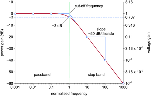
You can see in the graph that on the horizontal axis, the frequency scale is in a form that is known as logarithmic. What this means is that at equally spaced points instead of having 1, 2, 3 Hz etc., you have 1 , 10, 100 Hz etc. The frequency increases by a factor of 10 at each interval.

Secondly, the vertical axis shows the power gain, but is measured in decibels. This again is a logarithmic measure which is designed to measure the ratio of powers, but is probably more commonly known in the measurement of sound.

Just from the shape of the graph, it is clear that this gain function of a real filter is very different from the idealised ones that you saw earlier. For example, there is no sharp distinction between the passband and the stop band, and consequently no distinct cut-off frequency. By convention, the frequency at which the power gain drops 3 dB below the passband gain (or, in terms of voltage ratio, falls to 0.707 times the passband gain) is called the cut-off frequency, and this is true also for an active filter where the passband gain is likely to be other than 1.

In this normalised graph, the frequency axis is the normalised part. Notice that the frequency axis has no units, and the numbers on it are relatively low. (In electronics, such apparently low frequencies are seldom of interest; instead typically frequencies ranging from hundreds of hertz to gigahertz are more often used.) The normalised frequencies have been calculated by dividing actual frequencies by the cut-off frequency. This is why the cut-off point sits at 1 on the normalised frequency axis.

Dividing one frequency by another results in a pure number (that is, one without units), which is why the normalised frequency axis has no units. Similarly, dividing an output voltage by an input voltage produces a gain figure that also has no units. If the gain is converted to a decibel value, then strictly speaking that too has no units, although in Figure 9 ‘dB’ has been added after the number as though it were a unit as a reminder of the logarithmic nature of the function used.

As an example of how to translate normalised frequencies to actual frequencies, suppose a practical low-pass filter had a cut-off frequency of 10⁴ radians per second. Simply multiplying all the numbers on the horizontal axis of the normalised graph by 10⁴ and giving the unit as ‘radians per second’ would transform the graph into one showing gain against actual frequency for that particular filter. If the cut-off frequency were 10⁴ Hz (rather than radians per second), the procedure would be just the same: multiply all the numbers on the axis by 10⁴ and give the unit as Hz.

All first-order low-pass filters have a gain function of this shape and with these slopes. The passband gain might differ if the filter is active (that is, if it incorporates amplification). For first-order passive filters (that is, those without amplification) the passband gain cannot exceed 1.

Notice that as you move right along the frequency axis, the gain never reaches zero (that is, zero as a voltage ratio rather than as a decibel number). Zero gain would correspond to a negatively infinite number of decibels.

All real first-order filters (as opposed to ideal ones) lack a sharp cut-off frequency; in addition, low-pass filters never fully cut off, although if the gain is low enough you can regard it as having fallen to 0. Higher-order filters can give a sharper cut-off than a first-order filter, but the brick-wall cut-off of an ideal filter can never be achieved in practice.

As you move left along the frequency axis, each division is one-tenth of the one before, and this can continue indefinitely. A logarithmic frequency scale therefore never reaches a frequency of 0.

The steepness of the gain in the stop band is referred to as the filter’s roll-off. All first-order filters have a 20 dB/decade roll-off. The same roll-off can also be specified as 6 dB/octave. An octave is a term borrowed from music and represents a doubling of frequency. (It is so called because the frequency span in a doubling of frequency is divided into the eight notes of a musical scale.) Higher-order filters have a steeper roll-off. For second-order filters it is 40 dB/decade (or 12 dB/octave) and for third-order filters it is 60 dB/decade (or 18 dB/octave). Each successive order adds a further 20 dB/decade (or 6 dB/octave) to the roll-off.

Note that at the first decade above the cut-off frequency, the gain of a first-order filter is 20 dB below the passband gain, not 20 dB below the gain at the cut-off frequency.

Now have a go at Activity 5.

As you saw earlier, filters affect the gain and phase of a signal. In the next section you will see how you can show this in the Bode plot.