

2.6 The full Bode plot: gain and phase
In Section 2.5, you heard how a full Bode plot would show not only how the gain changes with frequency, but also how the phase difference between output and input changes with frequency. Conventionally the phase plot is put under the gain plot, with their respective frequency axes aligned, as in Figure 10. This example is for a first-order low-pass filter.
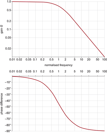
Figure 10 shows that in the passband, the output is virtually in phase with the input. As frequency increases towards the cut-off frequency (1 on the normalised frequency axis), a phase difference opens between the output and the input, with the output lagging the input (the negative values of phase angle indicate lagging phase). At the cut-off frequency, the phase difference is −45°. This means that for a sinusoidal input, the output lags the input by 45°. By the time you are well into the stop band, the phase difference levels off at −90°.
That concludes the discussion of first-order filters. To end Section 2 you will consider some commonly found higher-order filters and have a look at their characteristics.