3.7 Fourier transforms and the sinc pulse

You saw earlier (Figure 5) that the ideal frequency responses shown in Figure 22 are sometimes referred to as brick-wall filters because of the sharp transitions between passbands and stop bands. In other words, they are rectangular functions. However, whilst it is possible to use a rectangular function in the frequency domain to specify the filter, you must perform the calculations to implement the filter in the time domain. To do this, you need to translate between the time and frequency domains; in particular, for a brick-wall filter, you need to know what a rectangular function in the frequency domain looks like in the time domain. For a continuous-time system, you would use a Fourier transform to do this; for a discrete-time system, you use a corresponding discrete-time Fourier transform.

You can perform mathematical calculations on paper to work out the Fourier transform of a signal in either the time or the frequency domain. Under those circumstances, you would use the formula for either the discrete or the continuous transform, depending on the type of system you were dealing with. However, the majority of Fourier transforms will be carried out by a computer system – even if the system is dealing with continuous-time signals as input and output, the signal processing will be happening in the discrete-time domain of the computer. There is a particular algorithm called the fast Fourier transform (FFT) that is used to carry out Fourier transforms efficiently. Such was the need to perform these calculations at great speed that the FFT was included in a list of the top 10 algorithms of the twentieth century by the IEEE journal Computing in Science & Engineering in the year 2000 (Dongarra and Sullivan, 2000).

Using the discrete-time Fourier transform, you can see that the time-domain representation of a rectangular function in the frequency domain is the sinc pulse, as shown in Figure 24.

Figure 24 Fourier transform pair: a rectangular function in the frequency domain is represented as a sinc pulse in the time domain

Show description|Hide description

This figure consists of two graphs with a double-headed arrow in between them.

The graph on the left shows signal value against time. It is made up of a large number of vertical lines extending from the horizontal axis. If you were to join the ends of the lines, the shape would be a symmetrical curve consisting of a tall central peak with much smaller lobes on each side, alternating below and above the horizontal axis, and reducing in height the further away they are from the centre. This shape is known as the sinc pulse.

The graph on the right shows spectrum against frequency. It starts as a horizontal line close to 0, then rises vertically to a new value, where it stays for a certain range of frequencies before descending vertically back to nearly 0. The overall shape is that of a rectangle.

Figure 24 Fourier transform pair: a rectangular function in the frequency domain is represented as a sinc pulse in the time domain

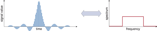
Mathematically, a sinc pulse or sinc function is defined as sin(x)/x.

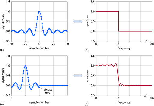
Figure 25(a) and Figure 25(b) show a sinc envelope producing an ideal low-pass frequency response. However, there is an issue because the sinc pulse continues to both positive and negative infinity along the time axis. Whilst mathematically you can readily take the Fourier transform of a sinc pulse, it can’t be computed because of the extension to infinity. The obvious solution is to truncate the sinc response as in Figure 25(c), so that the ripples no longer extend to infinity. Now that the pulse is finite, it can be shifted so that it only has positive sample numbers. The effects of this in the frequency domain are shown in Figure 25(d) – ripples in the passband and the stop band. In essence this shows why you can never have the perfect ideal or ‘brick-wall’ filter.

Figure 25 (a) Ideal sinc function in the time domain; (b) frequency response of the ideal sinc function; (c) abruptly truncated sinc function in the time domain; (d) frequency response of the truncated sinc function

Show description|Hide description

This figure consists of four graphs. Graphs (a) and (c) are time-domain graphs, showing signal value against sample number. Graphs (b) and (d) are frequency-domain graphs, showing spectrum against frequency. Graphs (a) and (b) are paired with a double-headed arrow, as are graphs (c) and (d).

Graph (a) shows samples that can be joined to make the shape of the sinc pulse from the previous figure: a symmetrical curve consisting of a tall central peak with much smaller lobes on each side, alternating below and above the horizontal axis, and reducing in height the further away they are from the centre. The curve is centred on sample number 0.

Graph (b), its frequency-domain equivalent, shows a graph line that takes a value of 1 at frequencies below f subscript c and a value of 0 at frequencies above fsubscript c, with a vertical drop from 1 to 0 at f subscript c.

Graph (c) has the same shape as in graph (a), but cut off abruptly after a couple of lobes on each side. It has then been shifted so that the left cut-off point is at sample number 0. All samples above the right cut-off point have a value of 0.

Graph (d), its frequency-domain equivalent, has a similar shape to graph (b), but there are oscillations around 1 below f subscript c and oscillations around 0 above fsubscript c. Also, the graph line no longer drops vertically at f subscript c, but falls diagonally from a frequency slightly below the cut-off to a frequency slightly above the cut-off.

Figure 25 (a) Ideal sinc function in the time domain; (b) frequency response of the ideal sinc function; (c) abruptly truncated sinc ...

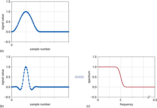
A technique for dealing with the truncated sinc is to apply a window function that brings the endpoints of the truncated sinc to zero. Figure 26(a) shows a suitable shape of window, Figure 26(b) shows the effects of applying the window to the truncated sinc and Figure 26(c) shows the resultant frequency response.

Figure 26 Using windowing to compensate for a truncated sinc pulse: (a) suitable window shape; (b) window applied to the truncated sinc; (c) resultant frequency response

Show description|Hide description

This figure consists of three graphs. Graphs (a) and (b) are time-domain graphs, showing signal value against sample number. Graph (c) is a frequency-domain graph, showing spectrum against frequency. Graphs (b) and (c) are paired with a double-headed arrow.

Graph (a) shows samples that can be joined to make a smooth, symmetrical bell-shaped curve that starts at 0 for sample number 0, then rises smoothly to a peak at signal value 1, then falls smoothly back down to 0. To the right of the bell-shaped curve, the value is 0 for all sample numbers.

Graph (b) shows samples that can be joined to make the shifted sinc pulse seen in Figure 6.12(c). Again, the left cut-off point is at sample number 0. However, the lobes have been reduced and smoothed out. The same thing has happened on the right-hand side, so that there is no longer an abrupt right cut-off point but a smooth transition from the reduced lobes into the zero values. The peak of the sinc pulse corresponds with the peak of the curve in graph (a).

Graph (c), its frequency-domain equivalent, is at a value of 1 for frequencies below f subscript c, with no oscillations. The graph line then falls diagonally from a frequency slightly below the cut-off to a frequency slightly above the cut-off. It remains at a value of 0 for frequencies above f subscript c, again with no oscillations.

Figure 26 Using windowing to compensate for a truncated sinc pulse: (a) suitable window shape; (b) window applied to the truncated sinc;...

When a window function is applied, it is effectively ‘multiplied’ with the sinc function. The process used to do this is called convolution. Convolution is outside the scope of this course, but when applied, what is left is where the signals overlap. You can think of this as a ‘view’ through the window function.

There are various shapes of window that can be applied. Two common shapes are the Blackman window and the Hamming window, although there are others (such as Kaiser, Bartlett and Hann). The Hamming window gives a better transition response, but the Blackman window has better stop-band gain and lower passband ripple.

You are now ready to design a digital filter and try it out.