
3.8 A low-pass filter design
You will now look at a real example of low-pass filter design. For this, a software package called Signal Wizard has been used. You are not required to download Signal Wizard, but for information, it is a free package that can be installed on your computer. Details of the Signal Wizard and where to find it are given can be found here: Installing Signal Wizard for use in offline mode [Tip: hold Ctrl and click a link to open it in a new tab. (Hide tip)] .
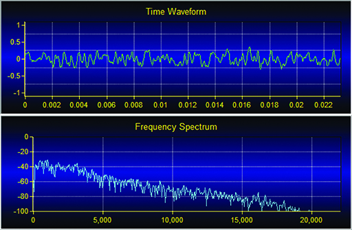
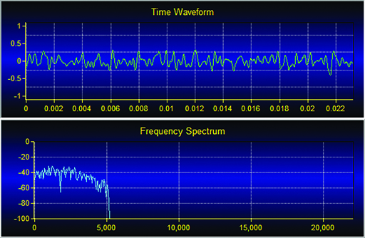
Figure 27 shows a screenshot from Signal Wizard which shows the input signal waveform both in the time domain (the ‘Time Waveform’) and in the frequency domain (the ‘Frequency Spectrum’). The aim is to remove any frequencies in this waveform above 5000 Hz, so a low-pass filter with a 5000 Hz cut-off frequency is required.
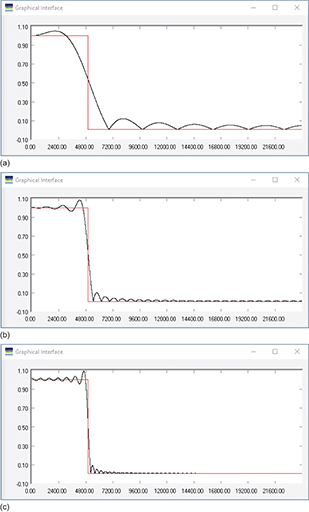
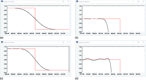
The specification of an FIR low-pass filter with a gain of 1 and a cut-off frequency of 5000 Hz is entered into the filter design interface. The graphical interface windows in Figure 28 all show the ‘brick-wall’ specification in red with the implementation in black. These designs all use a rectangular window, which gives an abruptly truncated sinc function. The first design uses 15 taps (Figure 28(a)), the second uses 63 taps (Figure 28(b)) and the third uses 127 taps (Figure 28(c)). All other parameters are unchanged. As the number of taps in the design increases from the top image to the bottom, the transition zone narrows and the designed filter more closely matches the filter specification. However, the amplitude of the ripples in the passband and the stop band remains unchanged, although the frequency increases as the number of taps increases.
The next set of designs, in Figure 29, keeps the number of taps at 127 and varies the window function used. The design implemented in Figure 29(a) uses a Blackman window, while the design implemented in Figure 29(b) uses a Hamming window. You can see that both have reduced the ripples in the passband.
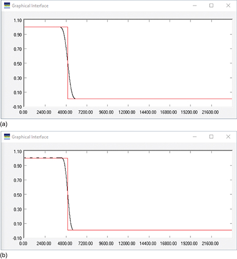
Figure 30 zooms in on sections of the transition band and passband to see the effects in more detail. Comparing Figure 30(a) and Figure 30(c) shows that the transition zone of the Hamming window is narrower than that of the Blackman window. Comparing Figure 30(b) and Figure 30(d) shows that the Blackman window has reduced the ripples in the passband more than the Hamming window. These results confirm that the Hamming window gives a better transition response, while the Blackman window has lower passband ripple.
The input signal was filtered using the 127-tap Hamming window design, and the output response is shown in the ‘Time Waveform’ and ‘Frequency Spectrum’ charts in Figure 31. The frequency spectrum shows that the filter has indeed taken out the redundant higher-order frequencies above 5000 Hz.
When a digital filter such as the one above is being implemented, the mathematical calculations will be defined in a software program, which will then run on some digital hardware. The basic processes taking place in the digital hardware are adding and subtracting; these processes will occur thousands, probably millions of times in the filtering of a sampled signal. Digital signal processor (DSP) chips are designed specifically to carry out these calculations, and their internal structure (referred to as their architecture) has been optimised to do so – thus it is different from that of a general-purpose processor used in a computer. There are several major DSP chip manufacturers, including Texas Instruments and Analog Devices.
You’ve therefore seen that usually a digital filter is designed using a software package. To finish this course, you will have a chance to explore digital filtering using an interactive resource. The next section introduces this resource.