
4.2.1 Quantifying thermal energy
Thermal energy is associated with random motion – that is, in effect, a definition. Because it is random, it only makes sense to talk about it in connection with a large population of atoms. I began with fifty million million million silicon atoms – that should be enough. If whatever motion they have is random, some may have lots of it, others very little. With such a large population it is reasonable to try to think about an average motion or, better, to define an average energy of the particles. How do you go about this?
Suppose that Figure 13(a) represents data about the time spent by Open University students on their tutor-marked assignments (TMAs) in all courses last year. The horizontal axis is the time, t, in minutes and the vertical scale is the number of students, N(t), taking a particular amount of time, t.
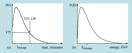
For any particular time on the horizontal axis you can use the curve to read off the number of students who took that long over their TMAs. Marked on the curve is the number of students who took between 125 and 126 minutes. To define the average time an Open University student spent on a TMA last year you must examine the statistics that the curve represents, showing, as it does, how the population is distributed among various time intervals. Then you refer to a mathematics text to advise you how to calculate the average from a statistical distribution. You can probably see by eye that the average lies a little to the right of the maximum in the curve.
The same approach ought to work for the average kinetic energy of a group of atoms. So let's look at the statistics of particle energies in a thermal distribution. It turns out that the statistical distribution of thermal energies among a large population of atoms (millions and millions of them) looks exactly like the curve I proposed for the TMA scores. I've sketched it again in Figure 13(b), with axes appropriately labelled. Now the vertical axis represents the number of particles having energies in any narrow interval on the horizontal energy axis. As with the TMA times, the average energy will be a little to the right of the maximum. I shall come to the mathematics of such distributions shortly.
Figure 13(b) represents a distribution of energies, with energy E plotted along the horizontal axis and the number N(E) plotted on the vertical axis. This distribution has a precise mathematical form that can be derived from a few fundamental principles and assumptions. It turns out that in this context, temperature expressed in energy units (kT, refer back to Box 2 Temperature and energy) is just a measure of average energy. So, a higher temperature corresponds with a distribution that has a higher average energy, and this would certainly be the case for one that has a broader distribution peaking at higher energy. There is a lot of thermodynamics behind these assertions. You must take this and what follows on trust if you have not met the idea before.