4.3.2 Competing processes
Let's look graphically at the way the rate of a thermally activated process changes with temperature. Figure 16 shows two rates with different activation energies of 1.0 and 0.5 eV – which curve is which?
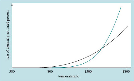
The process with the higher activation energy is the one that doesn't get going till the temperature gets up to around 1000 K, but once it has begun, it speeds up more quickly and, for the case illustrated, overtakes the process with the lower activation energy. It is sometimes like this with two thermally activated processes: at low temperature the lower activation process will predominate but above some temperature, the higher activation process may dominate proceedings.
This is worth remembering. If you are thinking of turning up the heat a little to hurry things along, take care not to unleash some other process with a higher activation energy of which you were previously unaware – I have in mind something like drying gunpowder with a blow torch!
Box 9 Carburizing steel
Here's a conundrum. Steel with a high carbon content is hard-wearing, and that is just what is required for drive-shafts, bearings and gear teeth. But if we choose a recipe that makes steel hard for a service requirement, how can we get around the fact that its hardness will make it extremely difficult to shape in the first place?
One answer is to fashion the components from a steel of a more formable, low-carbon composition and then increase the carbon content of the surface. That solves the problem, provided we can meet the challenge of squeezing extra carbon into the surface after shaping the components. That's where diffusion comes in.
Diffusion is spontaneous movement of matter caused by the thermal motion of atoms; it happens easily in gases and liquids, but in solids diffusion is a slow process. Nevertheless, the management of diffusion, as a means of altering the local composition of a solid material, is vital in many fields of engineering. Carbon is diffused into the surfaces of steel components to harden them and dopants are manoeuvred in silicon using diffusion to control semiconducting properties.
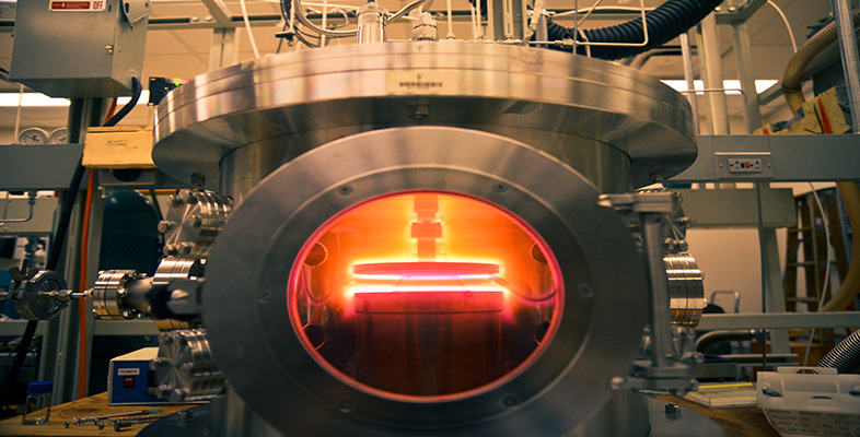
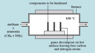
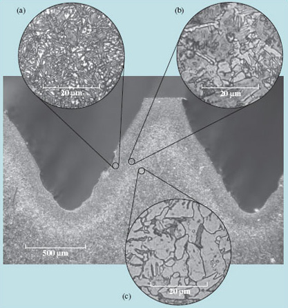
In solids, the kinetic energy is in the form of vibration, so on the whole nothing moves anywhere – except 'occasionally' when an atom manages to jump all the way from one lattice site to another. This possibility is thermally activated, with an activation energy that keeps the process virtually inactive at room temperature; diffusion in solids starts to be significant at temperatures of several hundred kelvin. Even when atoms do jump, they jump in random directions, so the overall travel of mass is very small. For example, in carburizing steel at 850 °C (about 1100 K) for 90 minutes, a typical treatment (Figure 17), it is estimated that each carbon atom has travelled over 100 m by making random hops from one space between iron atoms to another.
Yet, as shown in Figure 18, the carbon has penetrated less than 1 mm; there are nearly as many steps back as forward.
Whether or not there is any net flow by diffusion within the solid depends upon concentration gradients which lead to more hoppings in one direction than another.
Technologists are particularly interested in diffusion in non-uniform compositions, where the process is one of slowly changing concentrations at all places. Starting with an abrupt interface between two solids, the concentration profile after some time of diffusion must follow the trends of Figure 19.
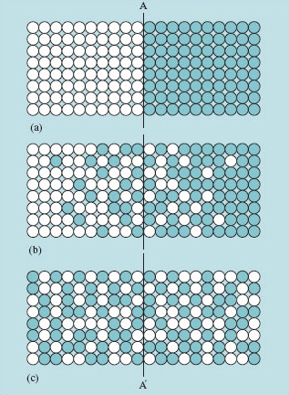
It is easy to see that the gradient of concentration encourages the change of composition. In Figure 19 random jumping will move more 'coloured' atoms across the plane A–A′ from right to left than the other way, simply because there are more of that species on the right of the plane. That reduces higher concentrations and raises lower ones until uniformity is reached. During the interesting transient phase, differential equations (proposed in the form of two laws by Adolf Fick in 1855) can relate concentrations to time and place via a diffusion coefficient:
in which Ea is the activation energy for the mechanism by which the atoms get to another site in the crystal, and D0 is the material property which converts the mere possibility of jumps (the exponential term) into an effect. The number of particles that are jiggling about with energies in excess of the strength of the bonds varies with the Arrhenius exponential.
To design a technical diffusion process an engineer has to determine how the concentration profile varies with time from some initial distribution. That involves solving Fick's Differential Equations. I'm not going to go into any more detail here, but what emerges are useful mathematical expressions for the concentration profile of the diffusing material. A useful rule of thumb coming from this solution is that the diffusing material has penetrated a distance ![]() after time t. But to use this result requires knowledge of D and of its temperature dependence; such data are catalogued for carbon diffusing in steel and for hundreds of other technically important combinations.
after time t. But to use this result requires knowledge of D and of its temperature dependence; such data are catalogued for carbon diffusing in steel and for hundreds of other technically important combinations.
Box 10 Thermistors
When metals get hot their electrical resistivity increases according to the linear model outlined in Section 3. Their conductivity (the reciprocal of resistivity) decreases with temperature. When ceramics get hot, although they're not noted for their electrical conductivity, they do the opposite and become better conductors of electricity at higher temperatures. Because they behave oppositely to metals, ceramics are sometimes said to have negative temperature coefficients (NTCs) for electrical resistance.
With a little ingenuity it's possible to make components for the electronics industry that can play the role of resistors while exhibiting this negative temperature coefficient behaviour. They can be used to compensate for thermal changes in the resistance of normal resistors. They can even be used as thermometers. These components are called thermistors.
A commonly used basis for thermistors is a mixture of manganese and nickel oxides. By controlling the gross composition and microstructure, components can be made with electrical resistances that change increasingly rapidly with temperature. The initial resistance, the resistance at a particular temperature and the rate of change with temperature can all be engineered to some degree.
'Microstructure' refers here to the size, shape and composition, on a microscopic scale, of distinct regions (such as individual crystals) in the bulk of the material.
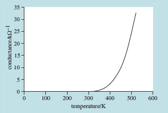
Figure 20 shows the reciprocal of the electrical resistance (electrical conductance) of one of a standard range of thermistors. Notice the rapid rise in conductance with temperature – just what you might expect when there's an exponential function involved.