4.2 The size of AGNs

AGNs appear point-like on optical images. It is instructive to work out how small a region these imaging observations indicate. Optical observations from the Earth suffer from 'seeing', the blurring of the image by atmospheric turbulence. The result is that star-like images are generally smeared by about 0.5 arcsec or more. One can do much better with the Hubble Space Telescope where, thanks to the lack of atmosphere, resolved images can be as small as 0.05 arcsec. What does this mean in terms of the physical size of an AGN?

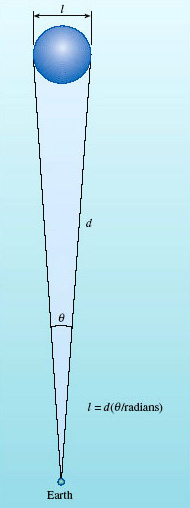
An arc second is 1/3600 of a degree and there are 57.3 degrees in a radian. So 0.05 arcsec corresponds to an angle of 0.05/(57.3 × 3600) rad = 2.4 × 10⁻⁷ rad. For such a small angle, the linear diameter of an object is related to its distance d by = d × θ, where θ is its angular diameter in radians (Figure 26).

Figure 26: Schematic diagram to show how the linear size ℓ of an AGN may be worked out from its angular size θ and distance d

The nearest known AGN is NGC 4395, a Seyfert at a distance of 4.3 Mpc and it, too, is unresolvable with the Hubble Space Telescope. So its linear size must be less than (4.3 × 10⁶) × (2.4 × 10⁻⁷) pc = 1.0 pc. So, for a nearby AGN, we can place an upper limit of order 1 pc on its linear size. (For a more distant AGN, this upper limit is correspondingly larger.) A parsec is a tiny distance in galactic terms. Even the nearest star to the Sun is more than one parsec away, and our Galaxy is 30 kpc in diameter. So the point-like appearance of AGNs tells us that they are much smaller than any galaxy.

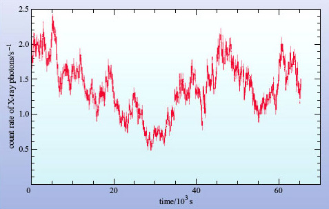
A second approach to estimating the size of an AGN comes from their variability. The continuous spectra of most AGNs vary appreciably in brightness over a one-year timescale, and several vary over timescales as short as a few hours (about 10⁴ s), especially at X-ray wavelengths (see Figure 27). This variability places a much tighter constraint on the size, as you will see.

J.C Lee et al., Astrophysical Journal, Volume 570, © 2002 The American Astronomical Society ©

J.C Lee et al., Astrophysical Journal, Volume 570, © 2002 The American Astronomical Society

Figure 27: An example of X-ray variability, shown by the Seyfert galaxy MCG-6-30-15 during an observation made by the Chandra X-ray Observatory. The fastest fluctuations are spurious noise, but the variability over a few thousand seconds is a property of the AGN

To take an analogy, suppose you have a spherical paper lampshade surrounding an electric light bulb. When the lamp is turned on, the light from the bulb will travel at a speed c and will reach all parts of the lampshade at the same time, causing all parts to brighten simultaneously. To our eyes the lampshade appears to light up instantaneously, but that is only because the lampshade is so small. In fact, light arrives at your eyes from the nearest point of the lampshade a fraction of a second before it arrives from the furthest visible point (Figure 28).

Figure 28: Light from the most distant visible point of a spherical lampshade will reach the observer a time R/c later than light from the near side. Fluctuations on timescales of less than R/c will not be observed

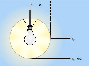
The time delay for the brightening, Δt, is given by

where R is the radius of the lampshade.

Now imagine the shade to be much larger, perhaps the size of the Earth's orbit around the Sun, and the observer is far enough out in space that the shade appears as a point source of light.

• What is Δt for a lampshade with the same radius as the Earth's orbit?

• Δt = (1.5 × 10¹¹ m)/(3 × 10⁸ m s⁻¹) = 500 s

So even if the lamp is switched on instantaneously, the observer will see the source take about eight minutes to brighten. Now suppose the bulb starts to flicker several times a second. What will an observer see? Even though the lampshade will flicker at the same rate as the bulb, it's clear that the flickering will have no effect on the observed brightness of the lampshade, since each flicker will take 500 seconds to spread across the lampshade and the flickers will be smeared out and mixed together. There is a limit to the rate at which a source (in this case the lampshade) can be seen to change in brightness and that limit is set by its size.

This argument may be inverted to state that if the observer sees a significant change in brightness of an unresolved source in a time Δt, then the radius of the source can be no larger than R = cΔt.

This kind of argument applies for any three-dimensional configuration where changes in brightness occur across a light-emitting surface. Of course, the argument is only approximate - real sources of radiation are unlikely to be perfectly represented by the idealised lampshade model that we have used here. The relationship between the maximum extent (R) of any source of radiation and its timescale for variability (Δt) is usually expressed as

(Where the symbol '∼' is used to imply that the relationship is correct to within a factor of about ten.)

Returning now to the AGN, let us calculate the value of R for an AGN such as MCG-6-30-15. The timescale for variability that we shall use is the shortest time taken for the intensity of the source to double. By inspecting Figure 27 it can be seen that this timescale is about 10⁴ s.

We have R ∼ cΔt, so with Δt = 1 × 10⁴ s, we obtain R ∼ 3 × 10¹² m = 1 × 10⁻⁴ pc. This is a staggeringly small result - it is ten thousand times smaller than the upper limit we calculated from the size of AGN images - and corresponds to about 20 times the distance from the Sun to the Earth. The AGN would easily fit within our Solar System. The argument does not depend on the distance of the AGN. Hence the observed variability of AGNs places the strongest constraint on their size.

One note of caution: the variability of AGNs usually depends on the wavelength at which they are observed. Variations in X-rays, for example, tend to be faster than variations in infrared light. Does this imply that the size of an AGN depends on the wavelength? In a sense, yes, as we are seeing different radiation from different parts of the object. The X-rays seem to come from a much smaller region of the AGN than the infrared emission, so we must be careful when talking about 'the size' of an AGN.

Question 7

An AGN at 50 Mpc appears smaller than 0.1 arcsec in an optical observation made by the Hubble Space Telescope, and shows variability on a timescale of one week. Calculate the upper limit placed on its size by (a) the angular diameter observation, and (b) the variability observation.

Answer

(a) An angular size limit of 0.1 arcsec corresponds to an angle in radians of

Multiplying this by the distance shows that the upper limit on the size is

(b) A week is 7 days which is 7 × 24 × 60 × 60 s. The upper limit from the variability is

(Thus variability constraints provide a much lower value for the upper limit to the size of the AGN than does the optical imaging observation.)

Other evidence also indicates the small size of AGNs. Radio astronomers operate radio telescopes with dishes placed on different continents. This technique of very long baseline interferometry (VLBI) is able to resolve angular sizes one hundred or so times smaller than optical telescopes can. Even so, AGNs remain unresolved.