1.6 Outline of the finite element analysis process: structural analysis
The number and type of elements chosen must be such that the variable distribution through the whole body is adequately approximated by the combined elemental representations. For example, if the mesh is too coarse, the resolution of the parametric distribution may be inadequate, whereas too fine a mesh is wasteful of computing time and possibly the user’s time, and in some cases, won’t even solve anyway. Part of the skill will be in designing and refining meshes in areas of high interest or concentration of results variation gradients.
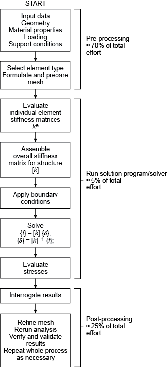
After model discretisation, i.e. subdividing the model domain into discrete elements (the mesh), the governing equations for each element are calculated and then assembled to give system equations. Once the general format of the equations of an element type (e.g. a linear distribution element) is derived, the calculation of the equations for each occurrence of that element in the body is straightforward. Nodal coordinates, material properties and loading conditions of the element are simply substituted into the general format. The individual element equations are assembled into the system equations, which describe the behaviour of the body as a whole. For a static analysis, these generally take the form , where, in structural problems, [ k ] is a square matrix, known as the global stiffness matrix, is the vector of unknown nodal displacements (or temperatures in thermal analysis) and is the vector of applied nodal forces (or heat flux in thermal analysis). The equation is directly comparable to the equilibrium or load–displacement relationship for a simple one-dimensional spring we invoked previously, where a force F produces or results from a deflection u in a spring of stiffness k . To find the displacement caused by a given force, the relationship is ‘inverted’, i.e. u = k −1f .
The same approach applies to the FEM using . However, before the equation can be ‘inverted’ and solved for , some form of boundary condition must be applied, as we’ve seen. In stress problems, the body must be restrained from rigid body motion. For thermal problems, the temperature must be defined at one or more nodes. The solution to the equation is not trivial in practice because the number of equations involved tends to be very large. It is not unreasonable to have 250 000 equations, and consequently [ k ] cannot be simply inverted – there is unlikely to be enough computer memory to store all the numbers and data.
Fortunately, as we’ve seen, [ k ] will probably be banded, i.e. terms are grouped about the leading diagonal of the matrix, and more ‘distant’ terms will be zero. Techniques have been developed to take advantage of these features to store and solve the equations efficiently without going through an ‘inversion’ process. Remember that we are generally solving for the nodal displacement values first; it is then a simple matter (using a computer package) to use the displacements to find the strains and then the elemental stresses, via the appropriate Hooke’s law and strain/stress (constitutive) relations.
The major stages in the creation of any finite element model, according to Baguley and Hose (1997), for most types of analysis are:
- selection of analysis type
- idealisation of material properties
- creation of model geometry
- application of supports or constraints
- application of loads
- solution optimisation.
It is extremely important to:
- develop a feel for the behaviour of the structure
- assess the sensitivity of the results to approximations of the various types of data
- develop an overall strategy for the creation of the model
- compare the expected behaviour of the idealised structure with the expected behaviour of the real structure.
For those of us who like pictorial representations, think of the process as shown in Figure 2. Note the estimated proportions of time and effort that are (or should be!) spent in the various phases of preprocessing, solution and post-processing.