Step 5 – Building and solving the FEA model

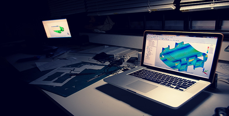
So the next task is to actually mesh the model. And that does take quite a while in this case because you need to make sure that all the elements are joined to one another at any of the geometry interfaces. So here we can see the final mesh, which is relatively fine for the size of the component. And this gives us a reasonable number of elements. I think there’s in excess of 20,000 per half on this model. And obviously that means, with the type of material that we use, that run times are actually a little larger than they would be for an isotropic model.

Before you solve the model, obviously, as always you need to check that the loads you’ve applied are what you expect. So you need to check your resultant forces in the package if it allows you to do so in the pre-processor. And make sure that all your restraints, and again constrain all six degrees of freedom, to stop there being any silly errors during the running.

Assuming that’s the case, you run the model and then look at the results. Now in the case of this component, and for this load case more specifically, we’re not really interested in stresses. Because it is literally just a stiffness check. The loads are all fairly arbitrary, just to allow us to calculate the stiffnesses more easily than normal.

Remember that Lewis set up the model as one half, considered symmetrical about the car longitudinal centre line. He used so-called quad four elements, which he considered adequate enough for determining overall tub stiffness, not being that interested in local stress gradient details. The trouble is, there were still 20,000 of them, even for just half the model. And what with the complications due to the material properties, significant computing time and resource is needed to solve the model. A model of the complete tub would need vastly more resource.

Notice that although the tub shape itself is symmetrical about the centre plane of the car, an anti-symmetry boundary condition was applied to the surfaces representing the cut between the two halves. This was because the loading on each half was not reflected as with a mirror but was equal and opposite due to the applied couple torsion action. Thus, an anti-symmetry boundary condition was necessary.

If we look at the six degrees of freedom for each node on the cut face, the x-axis is aligned with the car longitudinal centre line. The y-axis goes across the car, side to side. The z-axis is vertical.

For the anti-symmetry condition, the x and z directional degrees of freedom are constrained, as is the rotational degree of freedom about the y-axis. If the loading arrangement was also symmetrical, the symmetry boundary condition would be the exact opposite – constrain y displacement, constrain the rotations about the x and z axes.