5 Signal transmission

5.1 Transmission of electrical signals on wires

In the discussions of newsgathering in the Taylor and Higgins papers, you saw the significance of the development of systems that allowed long-distance transmission of electronic signals. Initially transmission used metallic wires (remember Taylor's reference to the importance of the 'lines infrastructure' and his mention of the 'wire picture') and later wireless transmission (terrestrial and satellite microwave) became important. In this section I shall look at some aspects of the transmission of digital signals, starting with a close look at the transmission of electrical signals on wires.

Using a wire to transmit a signal is simple in principle: you operate a switch at one place and observe the effect somewhere else. In Figure 17 I have shown this as a light coming on at a remote location. Notice in this diagram the standard symbol for a battery consisting of two parallel lines, one shorter than the other, and the symbol for a light bulb which is a circle with a cross in it. The standard symbol for a switch that can be 'open' or 'closed' consists of two dots and a line which either connects the dots (when the switch is closed as in Figure 17b) or misses one of the dots (when the switch is open, as in Figure 17a). To switch the light on you close the switch so that there is an electric circuit from the battery to the light bulb and back again. To switch the light off you open the switch to 'break' the circuit.

Figure 17 Switching a light on at a remote location: (a) light off; (b) light on

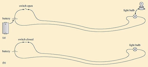
When you switch a light on, the light appears to come on immediately. There does not appear to be any delay between operating the switch and the effect at the light (although, depending on the type of light there might be a delay before it comes on fully – this is especially noticeable with fluorescent light tubes). In reality there is a delay – it is just very short indeed.

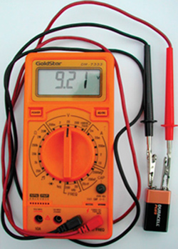
To get a better insight into what is happening, imagine measuring the voltage between the wires. This can be done with something called a voltmeter (Figure 18). A voltmeter has two wires and a display. When you touch the ends of the wires to the terminals of a power source like a battery, the display on the meter tells you what the voltage is between the terminals.

Maximise

Figure 18 A voltmeter

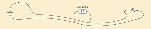
Imagine using the voltmeter to measure the voltage between the two wires at some point between the switch and the light, as in Figure 19. When the switch is open (off) the reading on the meter will be zero. When the switch is closed (on), the reading will (ideally) be equal to the voltage of the battery – which I shall assume is 1.2 volts. Now imagine having the voltmeter touching the wires while the switch is changed from open to closed. In this case you will see the voltage change from 0 to 1.2 V.

Figure 19 Measuring the voltage across a pair of wires

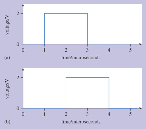
Now, if the voltmeter is touching the wires right next to the switch, you would see the voltage rise from 0 to 1.2 V at the same instant as the switch is closed. If, on the other hand, the voltmeter is touching the wires further away from the switch there will be a delay between the switch closing and the voltage rising. We can display this by plotting graphs as shown in Figure 20.

Figure 20 The voltage across wires when a switch is closed: (a) voltage across the wires as measured at the switch; (b) voltage across the wires as measured 200 m away from the switch

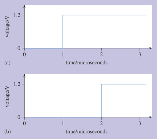
These graphs show how the reading on the voltmeter changes with time. Along the horizontal axis from left to right corresponds to time passing, and up the vertical axis corresponds to increasing voltage, as measured by the voltmeter.

The time axis is labelled in units of microseconds, where one microsecond is one-millionth of a second. Notice also that the time axis is relative to some time origin which is labelled 0. The actual time corresponding to 0 as shown on the axis might have been, say, Thursday 20 May 2004, 2.17 pm and 35.031233 seconds, but labelling the axis with that level of detail would be confusing and irrelevant.

Figure 20(a) shows what the voltmeter would do when connected to the wires next to the switch, while Figure 20(b) shows what it would do when connected to the wires 200 m along towards the light bulb. The switch was closed at time 1, on this scale, so the voltage measured next to the switch rises at time 1.

There is a delay before the voltage rises at the voltmeter when it is 200 m along the wire.

We can think of the change in voltage moving along the wires. This idea of the change in voltage moving along the wire becomes clear if we think about turning the light on and then off again afterwards. This is illustrated in Figure 21.

Figure 21 A voltage pulse travelling along a pair of wires: (a) voltage across the wires as measured at the switch; (b) voltage across the wires as measured 200 m away from the switch

Here, the switch is closed at time 1 microsecond and opened again at time 3 microseconds. We now have a voltage pulse. Looking at the voltage across the wires 200 m from the switch, both the rise and fall in voltage happen 1 microsecond later, and the voltage pulse has taken 1 microsecond to travel the 200 m along the wires.

This is two-thirds of the speed of light, which is typical of the speed that electric signals travel along wires.

Activity 27

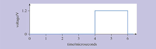
Assuming that the pulse continues to travel at the same speed, draw a graph of voltage against time for measurements taken 600 metres from the switch.

Discussion

The pulse travels 200 m in 1 microsecond, so it takes 3 microseconds to travel 600 m. The pulse will be as in Figure 22.

Figure 22 A pulse 600 metres along the wires, for the answer to Activity 27

Figures 20 and 21 (and my answer to Activity 27) are simplifications because they have not shown attenuation or distortion. Figure 23 shows the sort of effects that attenuation and distortion might have on a pulse.

Figure 23 Voltage across the wires as measured 200 m away from the switch, showing the effects of attenuation and distortion

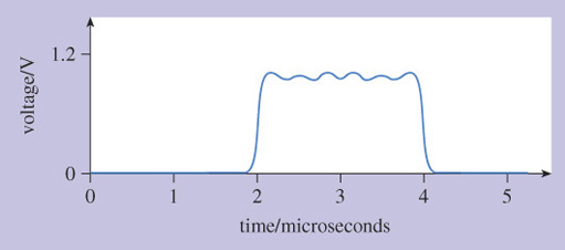
Attenuation reduces the height of the pulse, so that it does not reach 1.2 volts any more. Some of the voltage has been 'lost' as it travels the 200 metres because some energy from the electricity is absorbed by (very slightly) heating the wires and some energy is radiated into the air as the wires act as a (very inefficient) aerial.

Distortion alters the pulse, rounding the corners and generally changing the shape. Qualitatively, the smoothing of the corners is because the wires do not allow the voltage to change instantaneously – there is a sort of electrical drag as the pulse travels along the wires. More random distortion effects are caused by what is referred to as noise. By analogy with the common meaning of noise as unwanted, meaningless sounds, noise in the context of electrical signals is the unavoidable effect where signals develop unwanted, meaningless distortions.

Attenuation and distortion become worse as the pulse travels further. Amplifiers can be used to compensate for attenuation, but that still leaves distortion, which ultimately limits how far signals can be transmitted along a wire – or indeed any transmission medium. With digital signals, however, regenerators can be used instead of (or as well as) amplifiers to overcome both attenuation and distortion.

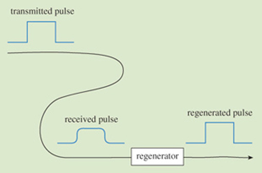
The concept of regeneration is that when a pulse has become badly attenuated or distorted, it can be regenerated to produce a new, perfect pulse for onward transmission. This is illustrated in Figure 24. Note that to simplify the diagram I have drawn a single line to represent a pair of wires. The pulses drawn next to the line represent pulses across the pair of wires at that location.

Figure 24 The concept of regeneration

You do not need to know how regeneration is done in detail; you just need to understand that it is possible. The reason it is possible is that with digital signals there is a restricted range of possibilities of what the signal could be. For example, with a binary signal, 1s and 0s might be transmitted on wire by using, say, 5 V to represent a 1 and 0 V to represent a 0. The regenerator 'knows' that the only signal it is expecting is something which started out either as a pulse of 5 V or as 0 V. The regenerator decides which of the two possibilities is most likely, and produces a new 5 V pulse or 0 V accordingly. Although there are practical complications, in principle this decision can be very simple. An electrical circuit compares the received voltage with a threshold value (say 2.5 V) and if the received voltage is greater than the threshold the output is a new 5 V pulse, otherwise the output is 0 V.

Ideally, regeneration can be repeated indefinitely allowing transmission over unlimited distances (Figure 25).

Figure 25 Successive regeneration for long-distance transmission

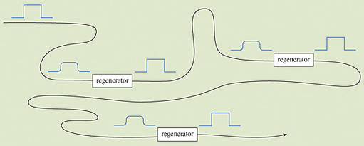
The boxes labelled 'regenerator' in Figure 25 are electronic circuits, but interestingly the very first 'regenerators' were human beings! Earl electric telegraph systems operated by the opening and closing of a switch at the transmitter having the effect of a pen putting marks on a piece of paper at the receiver. These were digital systems, with 'marks' and 'spaces' on the paper performing a similar role to 0s and 1s in modern digital systems. In telegraph relay stations, telegraph operators (people) would look at the marks and spaces on an incoming telegraph line and duplicate them on an outgoing telegraph to send the message on the next leg of its journey.