5.7 The standard deviation

The interquartile range is a useful measure of dispersion in the data and it has the excellent property of not being too sensitive to outlying data values. (That is, it is a resistant measure.) However, like the median it does suffer from the disadvantage that its calculation involves sorting the data. This can be very time-consuming for large samples when a computer is not available to do the calculations. A measure that does not require sorting of the data and, as you will find in later units, has good statistical properties is the standard deviation.

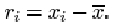
The standard deviation is defined in terms of the differences between the data values (x_i) and their mean . These differences , which may be positive or negative, are called residuals.

Example 1 Calculating residuals

The mean difference in β endorphin concentration for the eleven runners in section 1.4 who completed the Great North Run is 18.74 pmol/l (to two decimal places). The eleven residuals are given in the following table.

Difference, xi	25.3	20.5	10.3	24.4	17.5	30.6	11.8	12.9	3.8	20.6	28.4
Mean,	18.74	18.74	18.74	18.74	18.74	18.74	18.74	18.74	18.74	18.74	18.74
Residual,	6.56	1.76	−8.44	5.66	−1.24	11.86	−6.94	−5.84	−14.94	1.86	9.66

For a sample of size n consisting of the data values x ₍₁₎, x ₍₂₎, …, x_(n) and having mean , the ith residual may be written as

These residuals all contribute to an overall measure of dispersion in the data. Large negative and large positive values both indicate observations far removed from the sample mean. In some way they need to be combined into a single number.

There is not much point in averaging them: positive residuals will cancel out negative ones. In fact their sum is zero, since

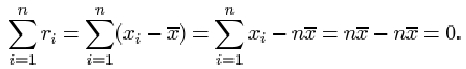
Therefore their average is also zero. What is important is the magnitude of each residual, the absolute difference . The absolute residuals could be added together and averaged, but this measure (known as the mean absolute deviation) does not possess very convenient mathematical properties. Another way of eliminating minus signs is by squaring the residuals. If these squares are averaged and then the square root is taken, this will lead to a measure of dispersion known as the sample standard deviation. It is defined as follows.

The sample standard deviation

The sample standard deviation, which is a measure of the dispersion in a sample x ₁, x ₂, …, x_n with sample mean , is denoted by s and is obtained by averaging the squared residuals, and taking the square root of that average. Thus, if , then

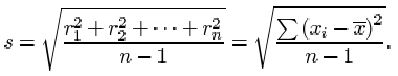
There are two important points you should note about this definition. First and foremost, although there are n terms contributing to the sum in the numerator, the divisor used when averaging the residuals is not the sample size n, but n−1. The reason for this surprising amendment will become clear later in the course. Whether dividing by n or by n−1, the measure of dispersion obtained has useful statistical properties, but these properties are subtly different. The definition above, with divisor n−1, is used in this course.

Second, you should remember to take the square root of the average. The reason for taking the square root is so that the measure of dispersion obtained is measured in the same units as the data. Since the residuals are measured in the same units as the data, their squares and the average of their squares are measured in the squares of those units. So the standard deviation, which is the square root of this average, is measured in the same units as the data.

Example 2 Calculating the standard deviation

The sum of the squared residuals for the eleven β endorphin concentration differences is

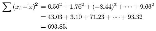
Notice that a negative residual contributes a positive value to the calculation of the standard deviation. This is because it is squared.

So the sample standard deviation of the differences is

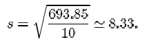
Even for relatively small samples the arithmetic is rather awkward if done by hand. Fortunately, it is now common for calculators to have a ‘standard deviation’ button, and all that is required is to key in the data. The exact details of how to do this differ between different models and makes of calculator. Several types of calculator give you the option of using either n or n−1 as the divisor. You should check that you understand exactly how your own calculator is used to calculate standard deviations. Try using it to calculate the sample standard deviation of the eleven β endorphin concentration differences for runners who completed the race, using n−1 as the divisor. Make sure that you get the same answer as given above (that is, 8.33).

You will find that the main use of the standard deviation lies in making inferences about the population from which the sample is drawn. Its most serious disadvantage, like the mean, results from its sensitivity to outliers.

Activity 13: Calculating standard deviations

In Activity 12 you calculated a standard deviation of 98.0 for the data on the collapsed runners. Try doing the calculation again, but this time omit the outlier at 414. Calculate also the interquartile range of this data set, first including the outlier and then omitting it.

Answer

Solution

When the outlier of 414 is omitted, you will find a drastic reduction in the standard deviation from 98.0 to 37.4, a reduction by a factor of almost three!

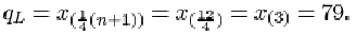
The data are given in order in Activity 12. For the full data set, the sample size n is 11. The lower quartile is

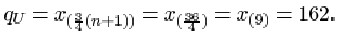
The upper quartile is

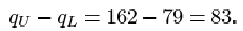
Thus the interquartile range is

When the outlier 414 is omitted from the data set, the sample size n is 10. The lower quartile is

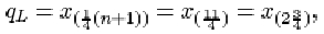
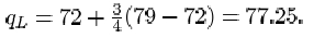
which is three-quarters of the way between x ₍₂₎=72 and x ₍₃₎ = 79. Thus

The upper quartile is

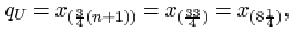
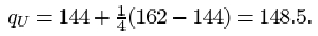
which is one-quarter of the way between x ₍₈₎=144 and x ₍₉₎=162. So

The interquartile range is

Naturally it has decreased with the removal of the outlier, but the decrease is relatively far less than the decrease in the standard deviation.

You should have found a considerable reduction in the standard deviation when the outlier is omitted, from 98.0 to a value of 37.4: omitting 414 reduces the standard deviation by a factor of almost three. However, the interquartile range, which is 83 for the whole data set, decreases relatively much less (to 71.25) when the outlier is omitted. This illustrates clearly that the interquartile range is a resistant measure of dispersion, while the standard deviation is not.

Which, then, should you prefer as a measure of dispersion: range, interquartile range or standard deviation? For exploring and summarising dispersion (spread) in data values, the interquartile range is safer, especially when outliers are present. For inferential calculations, which you will meet later in the course, the standard deviation is used, possibly with extreme values removed. The range should only be used as a check on calculations. Clearly the mean must lie between the smallest and largest data values, somewhere near the middle if the data are reasonably symmetric; and the standard deviation, which can never exceed the range, is usually close to about one-quarter of it.