

5.11 Numerical summaries: summary
In this section, various ways of summarising certain aspects of a data set by a single number have been discussed. You have been introduced to two pairs of statistics for assessing location and dispersion. The median and interquartile range provide one pair of statistics, and the mean and standard deviation the other, each pair doing a similar job. As for the choice of which pair to use, there are pros and cons for either. You have seen that the median is a more resistant measure of location than is the mean, in the sense that its value is less affected by the presence of one or two outliers in the data. In the same sense, the interquartile range is a more resistant measure of dispersion than is the standard deviation.
The (sample) median is the central value in a data set after the data values have been sorted into order of increasing size. The lower and upper (sample) quartiles are the values that divide the data set into quarters. Denoting by x (p) the pth value in the ordered data set of n values, the median to, the lower quartile qL and the upper quartile qU are given by
m = x (½(n+1)), qL = x (¼(n+1)), qU = x (¾(n+1)).
In each case, if the subscript is not a whole number, it is interpreted by interpolating between sample values. The interquartile range is q U −q L . A much less commonly used measure of dispersion is the range, which is simply the difference between the largest and smallest values in the sample.
No sorting of the data is required when calculating the (sample) mean and (sample) standard deviation. The mean x and the standard deviation s of a sample x 1, x 2,… x 1 are given by
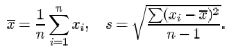
The variance is the square of the standard deviation.
The term ‘mode’ can be used to describe a ‘representative value’ in a data set; it describes the most frequently occurring observation. For numerical data, this definition needs to be modified; a mode is taken to be a clear peak in a histogram of the data. Some data sets have only one such peak and are called unimodal, others have two peaks (bimodal) or more (trimodal, multimodal).
Finally, you have learned to distinguish between data sets that are symmetrical, right-skew (or positively skewed, with a long tail of high values) and left-skew (or negatively skewed, with a long tail of low values). The sample skewness is a numerical summary of the skewness of a data set.