4.7 The global ocean circulation

As seawater freezes and ice is formed in the annual cycles you saw in Activity 2, salt is squeezed from between the ice crystals into the ocean beneath in a process called salt rejection. The result is that if you took one pancake ice floe (Figure 21b) and melted it in a bucket, the water that resulted would be fresher than the seawater you started with. So what has happened to the salt?

The answer is it has increased the density of the seawater just beneath the ice. This is a small-scale physical process, but the effects are global and profound, as is clear from Figure 13. Salt rejection from sea ice generation in the Antarctic creates dense water which sinks and floods away from the continent. The coldest water is not the most saline; it is the combination of the cold temperatures and increased salinity that makes the water dense enough to sink to the sea floor.

The very large volume of water of uniform temperature and salinity flooding away from Antarctica is called Antarctic Bottom Water (AABW) because it is formed in the Antarctic and is dense enough to reach the bottom of the ocean and flow away from the continent. The lowest-salinity water at ~1000 m depth and ~40° S, coloured purple and blue in Figure 13, is formed by the climatic conditions in the mid-latitudes of the Southern Hemisphere and is not as dense as AABW.

You have investigated a section through the Atlantic Ocean, but had you looked at any section radiating from Antarctica along a particular longitude, the picture would have been broadly similar. The sea ice generation and resulting salt rejection is driving a cold, relatively salty, dense water current northwards along the sea floor at great depth.

If a deep, cold, salty current is flowing away at depth, there has to be water flowing towards Antarctica to replace it. Arctic salt rejection increases the density of the waters at the other end of the planet but, because of the shallow sea floor between Greenland, Iceland and the UK, the densest water is contained and cannot flow south. What can escape into the North Atlantic sinks to the sea floor, and so is called North Atlantic Deep Water (NADW). The resulting picture of ocean circulation in the Atlantic when these water masses meet is shown in Figure 23.

Maximise

Figure 23 A schematic cross-section of the circulation in the Atlantic Ocean. Colours represent different water masses and blue arrows represent their movement. The AABW is dense enough to fill up the deep basins of the South Atlantic. The NADW is less dense and so it rises up over the AABW and fills up the mid-depths of the South Atlantic when the water masses meet.

Show description|Hide description

This chart shows major flows and water masses.

The horizontal axis is unlabelled but is marked in units of degrees latitude, from 80 degrees south (Antarctic) to 80 degrees north (Arctic), at intervals of 20 degrees, with the Equator marked at zero degrees.

The vertical axis is labelled 'depth' and is marked in units of metres, from zero to 6000, at intervals of 1000 metres beginning at the top.

The water masses and flows are complex, but two main water masses are labelled:

1. The AABW. The upper boundary of this mass descends fairly steadily from around 500 metres depth at 75 degrees south to around 4500 metres depth at the Equator. Its lower boundary descends sharply to around 5200 metres at 60 degrees south then fluctuates between approximately 4500 and 5800 metres, linking with the upper boundary at the Equator. Within the AABW, the main flow follows the lower boundary from the Antarctic to the Equator with a rising branch at around 50 degrees south creating a vertical circulation.
2. The NADW. The upper boundary fluctuates between 2000 metres depth at 50 degrees south, reaching the surface at approximately 60 degrees north. This lower boundary descends evenly to 5800 metres at 30 degrees north, then ascends to 1500 metres in the Arctic. Within the NADW, the main flows are southwards at various depths, with some northward flow at depth between the Equator and 30 degrees north.

Figure 23 A schematic cross-section of the circulation in the Atlantic Ocean. Colours represent different water masses and blue arrows ...

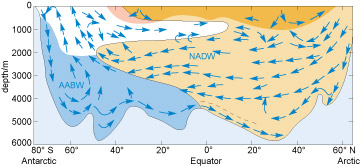
The dense AABW (coloured blue) spreads northwards along the sea floor and the NADW (brown) spreads south.

Figure 24 shows that NADW is both warmer and more saline than AABW, so it is less dense (Figure 23). However, the NADW is denser than the water mass coloured white and consequently is sandwiched between this and the AABW.

The actual boundaries between the layers are not as distinct as the colours in the picture would suggest, but overall there is an overturning circulation along the length of the Atlantic Ocean. In the Pacific and Indian Oceans the picture would be similar to Figure 23 south of the Equator, but the northern end would be different.

The Indian Ocean does not reach the Arctic, and in the Pacific Ocean, as you have seen, the gap between Asia and North America is so narrow and shallow that the ocean is virtually closed off to the north. This means that virtually all of the deep waters formed in the Arctic enter the global ocean in the North Atlantic. The result is a vast three-dimensional circulation across the entire global ocean called the thermohaline circulation ('thermohaline' meaning heat and salt) (Figure 24). This was proposed in the 1980s by American climate scientist Wallace Broecker. It is often referred to as the 'conveyor belt'.

Figure 24 A schematic diagram of the thermohaline circulation that moves both heat and salt around the planet. A large component of the forcing in this conceptual circulation is coming from processes happening in the Arctic and the Antarctic.

Show description|Hide description

This chart shows a map of the world with major oceanic flows superimposed.

The horizontal axis is unlabelled but is marked in units of degrees longitude, from 60 degrees west to 120 degrees east, at intervals of 60 degrees, with tick marks every 20 degrees. The midpoint is at 120 degrees east corresponding approximately with the west coast of Australia.

The vertical axis is unlabelled but is marked in units of degrees latitude, from 60 degrees north to 60 degrees south. The only others latitudes labelled are 20 degrees north and south, and the Equator at zero degrees; all three of these are shown as lines of latitudes across the width of the map.

Labelled 'warm upper waters', one flow is shown rising in the North Pacific (approximately 30 degrees north, 180 degrees east), flowing south where it splits into two at the Equator. One branch flows south then east around the tip of South America, turning north into the South Atlantic to meet the other branch which flows west between Australia and South-East Asia then around the southern tip of Africa. From here it flows north, descending at approximately 70 degrees north, zero degrees east. Another rising flow meets this westward branch in the Indian Ocean.

This descent links to the flow labelled 'cold deep and bottom waters', flowing south in the Atlantic then turning east at approximately 50 degrees south, 30 degrees west. From here it splits into two. The main branch flows past Antarctica, turning north near New Zealand at approximately 50 degrees south, 180 degrees east, rising to meet the warm surface flow mentioned above. The smaller branch flows north-east into the Indian Ocean where it rises and completes the circulation.

Figure 24 A schematic diagram of the thermohaline circulation that moves both heat and salt around the planet. A large component of the ...

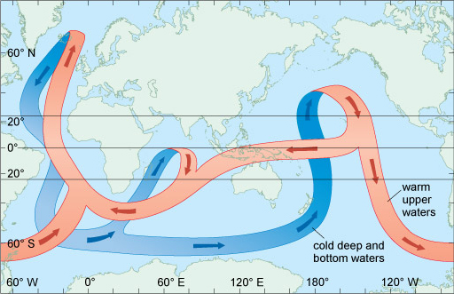
Figure 24 is of course a gross simplification, but it is useful to help you think about the way the global ocean circulates over hundreds of years. It makes clear that polar processes such as the sea ice growth can drive the global ocean circulation and move vast quantities of heat and salt around the planet. Ultimately it is these processes that are responsible for the sea surface temperature distribution you saw in Figure 1, making the UK and Norway warmer than locations at similar latitudes on the west side of the Atlantic.