6.4 Government expenditure (4)

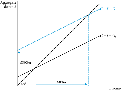
The aggregate demand model can also be used to illustrate what might happen under an increase in government spending, as shown in Figure 15. Let government spending increase by £300 million – money that could be spent along the lines of the 2009 Obama Recovery Act or the 1929 Lloyd George three-point plan. This is shown by an upward shift of the intercept of the aggregate demand schedule by £300 million due to an increase in government spending from G₀ to G₁. It is referred to in modern economics as a fiscal stimulus. Using one of its key fiscal powers – the ability to carry out expenditure – the government is able to boost aggregate demand.

Figure 15 Modelling a fiscal stimulus

Show description|Hide description

This diagram has Aggregate Demand (AD) on the vertical axis and Income (Y) on the horizontal axis.

A solid line at a 45 degree angle is drawn upwards from the origin.

From a short way up the vertical axis, a straight line is drawn, sloping upwards at an angle shallower than 45 degrees. This line is labelled as C+I+G zero and it intersects the 45 degree line quite low down. A dashed line is drawn from this intersection point down to the horizontal Income axis.

From a point about half way up the vertical axis, a second straight line is drawn. This is parallel to the first one and is labelled as C+I+G1. This intersects the 45 degree line much further along. A dashed line is drawn from this intersection point down to the horizontal Income axis. This point is much further along the axis than the point from the first aggregate demand schedule.

There are two arrows in blue showing the direction of change. One arrow points upward along the vertical axis, from the lower to the higher aggregate demand schedule. This has £300m written beside it.

Another arrow runs to the right along the horizontal axis, from the lower point on the axis to the higher point. This has £600m written beside it.

Figure 15 Modelling a fiscal stimulus

This ‘double your money’ insight can now be explained by breaking down the effect of the stimulus into a series of rounds, as shown in Table 1. In Round 1, the change in income is equal to the fiscal stimulus of £300 million. Round 2 then depends on how much of this income is spent.

It is modestly assumed in Figure 15 that the marginal propensity to consume – the slope (b) of the consumption function – is equal to 1/2. This means that in Round 2, half of the initial increase in income from the fiscal stimulus will be spent on consumption, as shown by the £150 million change in income. By Round 2 it therefore follows that there is a cumulative increase in income of (i) the initial direct increase in income of £300 million, and (ii) the additional indirect impact of £150 million. These two items add up to a cumulative income of £450 million in Round 2.

This process continues in Round 3, with half of the previous round’s change in income (£150 million) spent as consumption: a new change in income of £75 million. In each round, half of the previous round’s change in income is spent; these rounds continue indefinitely. By Round 10, however, the change in income has fallen to just over half a million pounds, and the cumulative change approaches its final value of £600 million – the doubling of income that is illustrated in Figure 15. Even by Round 3, 87.5% of the eventual cumulative change in income has occurred, so although in theory the expansionary effect may take many rounds and a great deal of time to work itself out, the main impact is felt quite quickly.

Figure 16 shows the first three rounds. In Round 1, the injection of government demand leads to an upward shift of the aggregate demand schedule by £300 million. Initially, this planned aggregate demand exceeds current output. At the outset, in Round 1, only £200 million worth of output (income) is being produced, yet now the total aggregate demand is £500 million. If the key assumption is now made that there is sufficient spare capacity – idle factories or machinery, and a pool of unemployed workers – then in response to the additional demand, output can be increased by £300 million, as depicted by the first horizontal arrow.

Figure 16 Direct and indirect impacts of a fiscal stimulus

Show description|Hide description

This diagram has Aggregate Demand (AD) on the vertical axis and Income (Y) on the horizontal axis.

A solid line at a 45 degree angle is drawn upwards from the origin.

From a short way up the vertical axis, a straight line aggregate demand schedule is drawn, sloping upwards. This is labelled as C+I+G zero. This has a shallower slope than the 45 degree line and intersects the 45 degree line quite low down. A dashed line is drawn from this intersection point vertically down to the £200m point on horizontal Income axis.

From about half way up the vertical axis, a second aggregate demand schedule is drawn. This is parallel to the first one. This is labelled as C+I+G1. This intersects the 45 degree line much further along the line. A dashed line is drawn from this intersection point down to the horizontal Income axis. This point is much further along the axis than the point from the first aggregate demand schedule.

The diagram shows three rounds of the fiscal stimulus process, via a series of vertical and horizontal arrows that form three steps. The arrows decrease in length as we move from left to right.

The first vertical arrow runs from the point of intersection between the lower aggregate demand schedule and the 45 degree line directly up to the higher aggregate demand schedule. This has ‘£300m’ written beside it. . Above the point where the arrow hits the higher aggregate demand schedule is written ‘Round 1’.

From the point where the vertical arrow hits the higher aggregate demand schedule, an arrow runs horizontally right to hit the 45 degree line. This arrow has ‘£300m’ written beside it. Another arrow runs vertically up from this point on the 45 degree line up to the higher aggregate demand schedule, with ‘£150m’ written beside it. Above this point is written ‘Round 2’.

From this point on the higher aggregate demand schedule an arrow runs horizontally right to the 45 degree line, and then vertically up to the higher aggregate demand schedule. This has ‘£75m’ written beside it and above is written ‘Round 3’. A final short arrow is drawn horizontally to the 45 degree line. This is just short of the equilibrium position, where the higher aggregate demand schedule intersects the 45 degree line.

There is one further line on the diagram. From the point where the first vertical arrow hits the higher aggregate demand schedule, a dashed line is taken horizontally left to the vertical axis, to a point labelled ‘£500m’

Figure 16 Direct and indirect impacts of a fiscal stimulus

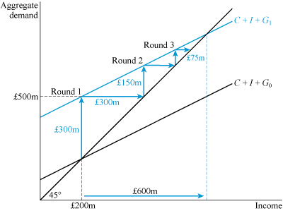
In Round 2, the new stimulus of £150 million, as shown in Table 1, comes into play. Once again aggregate demand exceeds current output, this time by £150 million, and a new horizontal line indicates the increase in output to match this demand. Similarly, in Round 3 the impact of the £75 million boost in aggregate demand is matched by a £75 million boost in output. These rounds eventually peter out, as in Table 1, when both aggregate demand and aggregate output have increased by £600 million.

The process, illustrated in Table 1 and in Figure 16 is referred to by Keynes as the multiplier process, since the impact of the fiscal stimulus is multiplied throughout the economy. The multiplier captures the cumulative effect of a change in spending on income. The change represented here is a change in government spending, but the model could also be used to show the effect of a change in another exogenous factor such as investment.

Let Δ denote the amount by which a variable might change. The multiplier can be expressed in mathematical terms as the ratio of the eventual change in income (ΔY ) to the initial change in spending that caused it (ΔG ):

The size of the multiplier depends on the marginal propensity to consume, as explored in the box below. It has a simple formula:

where b is the marginal propensity to consume. In the example in Table 1, the propensity to consume is equal to 1/2. Hence

The eventual doubling of income in the multiplier process is captured in total by this formula for the multiplier.

Since the concept of the multiplier emerged in the 1930s, economists have used statistical methods to estimate its empirical size. There is, however, considerable uncertainty as to the multiplier’s precise value. At the top end of estimates of the size of the multiplier, Eggertsson (2006) finds the multiplier to be as high as 3.8. In a more recent survey, Ramey (2011) pronounces that the ‘range of plausible estimates for the multiplier … is probably 0.8 to 1.5’. Due to the uncertainty involved, however: ‘Reasonable people could argue that the multiplier is 0.5 or 2.0’. A multiplier of 0.5 would mean, for example, that £1 billion of spending leads to only half that increase in income; whereas a multiplier of 2.0, as you have seen, would mean a doubling of income.

One problem is that estimates tend to be based on observations made during periods of economic growth, yet multipliers are most relevant in times of contraction. Larry Summers, a leading US economist who has advised Presidents Clinton and Obama, has been very cautious about the impact of fiscal stimuli but argues that the specific circumstances of the economic crisis of 2008 would point to a multiplier nearer to the top end of Ramey’s range of estimates (DeLong and Summers, 2012).