Long run average cost (LRAC) curves

In the long run it is possible to change all the inputs used in production. The long run average cost curve shows the average cost for the firm at a range of different levels of output. The firm can potentially reduce costs from:

• economies of scale
• technological change
• learning by doing.

The figure below summarises these three channels of cost reduction.

Figure 29 Two LRAC curves

Show description|Hide description

This diagram has ‘Cost’ on the vertical axis and ‘Quantity’ on the horizontal axis.

It shows two very shallow U shaped curves, one just above the other. The upper curve is labelled ‘LRAC1’. The lower curve is labelled ‘LRAC2’. The lowest sections of both curves are actually quite flat for a long section before rising again. The upward rising section of both curves is very short.

Three points are marked on LRAC1. Point A is marked about half way along the downward sloping section of the curve. Point B is marked at the lowest point of the curve. Point C is marked on the upward rising section of the curve.

Three points are also marked on LRAC2. Point D is marked about half way along the downward sloping section of the curve. Point D lies directly below point A on LRAC1. Back on LRAC2, Point E is marked at the start of the flat lowest part of the curve. Point F is marked on the upward rising section of the curve.

Figure 29 Two LRAC curves

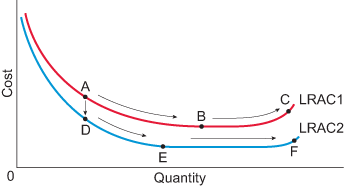
A firm moving from point A to B is a clear example of economies of scale: average cost falls as output increases. If the firm were on LRAC 2, then moving from D to E would also be an example of economies of scale.

Note that learning by doing cannot be shown on Figure 30. All LRACs (like the curve used above) show output for a given period of time on the horizontal axis. However, learning by doing is gained from cumulative experience of production, which is gained over time, not necessarily as a result of increasing output per day or per year.

From point A to point D, the firm’s LRAC has shifted downwards, so it is an example of technological change. Note in this example, at any output the firm’s average cost is lower having shifted to LRAC 2 compared to LRAC 1.

Diseconomies of scale only occur when a firm experiences increases to average cost as output rises. This occurs on LRAC 1 as the firm moves from B to C, and on LRAC 2 as the firm moves from E to F.

Each of the LRAC curves shown have a point which identified the minimum efficient scale (MES). For LRAC 1, this is point B, and for LRAC 2, this is point E. The MES occurs at the lowest level of output where average cost is at a minimum.