Short run cost curves (3)
Activity 23b
This time, click on the quantity axis in the figure to identify the level output where the difference between average cost and average variable cost is smallest.
Active content not displayed. This content requires JavaScript to be enabled.
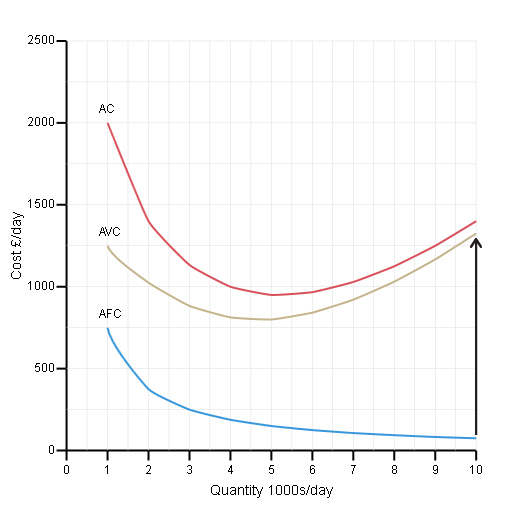
Figure 39 Average cost curves (3)
Interactive feature not available in single page view (see it in standard view).
Discussion
The difference between average cost (AC) and average variable cost (AVC) is least when output is high, in this case at a quantity of 10 000/day (see the black arrow on the figure below). This is the same as spotting that average fixed costs (AFC) are lowest when output is high, because: AC – AVC = AFC. In the short run, if output were to continue to increase beyond a quantity of 10 000/day then we would expect AFC to become smaller and smaller, and so make a smaller and smaller contribution to AC.