Pioneers
10. Theory of Computation
10.1. Vladimir Lukyanov
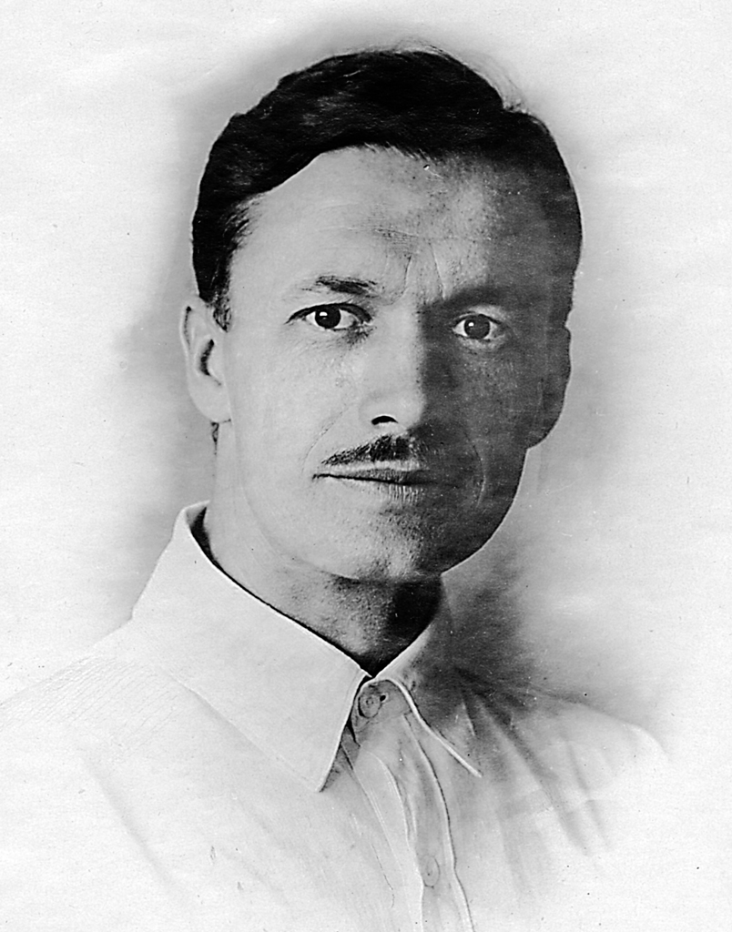
Figure 1: Vladimir Lukyanov
Source: Wikipedia (2015)
Downloadable teaching resource
Overview
Vladimir Sergeevich Lukyanov (Владимир Сергеевич Лукья́нов) was a Soviet engineer and inventor credited with creating the world’s first modern hydraulic analog computers. In 1936, he constructed the first of a series of “Water Integrators”, machines that used the flow of water through a network of tubes and chambers to solve partial differential equations.
Background
Vladimir Lukyanov was born in Moscow, the Russian Empire in 1902. He graduated from Moscow Classical Gymnasium in 1919 and joined the Moscow State University of Railway Engineering, graduating in 1925. Starting as a junior engineer he quickly advanced to the head of the technical department, becoming more involved with the planning and execution of the railway construction. In 1930 he went on to join the Central Institute of Railway Engineers, researching how to calculate the temperature inside concrete structures, especially in colder weather. It was in pursuit of a more accurate solution to the resultant complex differential equations that he started considering building a machine (Computer Timeline, no date).
Contributions
While he was working at the Central Research Institute of Building Structures in Moscow, Vladimir Lukyanov successfully designed the first hydraulic model to solve the issue of concrete temperatures in 1935, and his more advanced one-dimensional Hydraulic Integrator – for a wider class of differential equations - was developed in 1936.
The Water Integrators used a system of interconnected glass vessels, valves, and tubes through which water flowed to simulate and solve complex partial differential equations. Over the coming years Lukyanov would create two-dimensional and three-dimensional hydraulic integrators, allowing for ever more complicated mathematical equations to be modelled (Computer Timeline, no date).
Beginning in 1941, the machine was mass-produced and deployed across primarily Soviet institutions but also exported as far as China. They were used not only in construction science but also in metallurgy, thermodynamics, and rocketry. Some units remained in use into the 1990s, which attests to the device’s long-term scientific value and mechanical resilience (Manokhin, 2025).
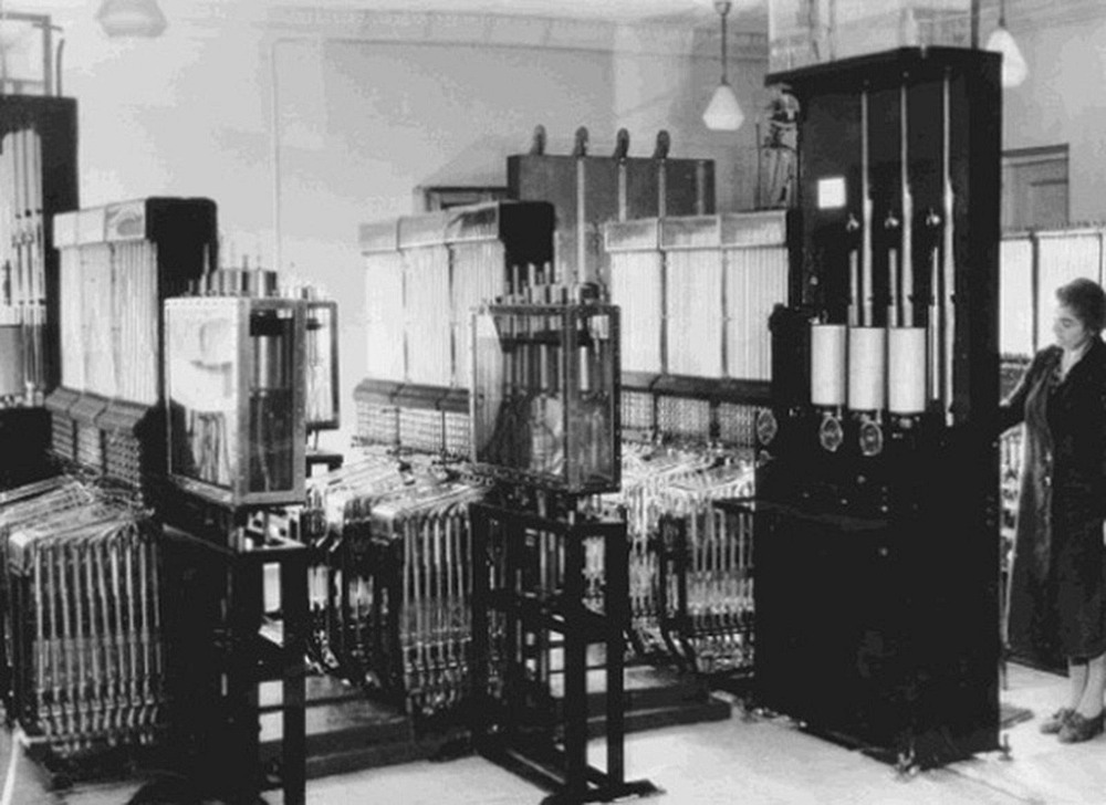
Figure 2: Lukyanov’s three-dimensional water integrator (AmusingPlanet, 2019)
Feature: The Water Integrator
After Lukyanov confirmed that the laws of water flow and heat dissipation are similar enough for modelling purposes he created the Water Integrator, initially from just roofing iron, tin, and glass tubes.
The main elements were the open-topped vertical vessels with a fixed capacity which were connected by tubes that varied in their hydraulic resistance. Raising and lowering the connected vessels of these tubes adjusted the water pressure.
The water levels in the vessels represented stored values, including the temperature difference between the air and material and the heat capacity of the material, and the flow rate, affected by hydraulic resistances that referred to thermal resistance, reflected the mathematical operations (Habr, 2025).
Watch
A short video documentary discussing the engineering problems Lukyanov set out to solve, and his solutions:
Video 1: The Soviet computer that used water to do math (Engineering History, 2020)
Transcript
During the 1920s and 30s the Soviet Union experienced rapid industrialization under Joseph Stalin's first five-year plan.
Due to Russia's vast distances a key component was the expansion of the rail network.
For the first five-year plan the Soviets aimed to add 17,000 kilometers of new rail to their existing network of 76,000 kilometers.
Building these rail lines was not only time consuming, but their quality was rather poor as the concrete used in construction had a tendency to crack.
One of the men working on this project was Vladimir Sergievich Lukyanov.
Born in 1902 and graduating from the Moscow institute of railway engineering in 1925 Lukyanov worked on various construction projects during the five-year plan.
By 1930 he was promoted to senior engineer at the central institute of construction of the People's Commissariat of Transport.
His interest at the time was to better understand the problem of concrete cracking - he believed that temperature was primarily responsible.
While his colleagues were apprehensive of this idea Lukyanov’s research into temperature and heat led him to complicated partial differential equations describing thermal systems.
Differential equations are equations which contain a function along with how the function changes.
They're very useful for describing systems found in the real world.
Here's a very basic example: it simply states that the rate of change of a function at a given point in time is equal to the value of that function at the same point in time.
The function itself is unknown and must be calculated using various techniques the main one being calculus.
The solution to this problem is shown here.
The C is an arbitrary constant.
This is because solving a differential equation usually leads to a family of solutions.
If we have some more information such as initial conditions we would be able to find an exact function.
This is an example of an ordinary differential equation, meaning it only changes with respect to one variable time in this case.
Partial differential equations on the other hand are much more difficult to solve as they deal with multiple changing variables, usually time along with dimensions in space.
This is the one-dimensional heat equation.
It describes how temperature changes over time in space in one dimension.
The C here is a constant which represents the properties of the medium.
Getting back to Lukyanov, he would have been interested in solving three-dimensional heat equations.
Unfortunately he lacked fast and precise methods to solve them.
There is one more thing we should discuss before getting to Lukyanov’s solution: interactions in a thermal system are invisible to the naked eye.
It is possible to describe and model them using partial differential equations though as I just mentioned there was no reliable way to do this in the early 1930s.
What if you could use a different physical system to model thermodynamics.
Consider this: heat flows from hot to cold just as water flows from high pressure to low pressure, the major difference being that it is much easier to measure and calculate water flow versus heat flow.
In 1934 Lukyanov set out to build a hydraulic computer observe its behavior and apply it to the world of thermodynamics.
In the following year he had created a basic prototype and by 1936 his device known as the hydraulic integrator was ready.
It was made up of mostly metal and various glass containers for water interconnected with multiple tubes with adjustable hydraulic resistances.
It was used in the falling manner - the user would set up the hydraulic integrator in a way that would reflect the thermal system in question.
For example: a container's cross-sectional area would correspond to a material's heat capacity, adding water to it would represent adding energy and the water level in the container would correspond to the object's temperature.
A second container with a different cross-sectional area could then represent a separate object with a different heat capacity.
By connecting these two containers and observing how water flowed between them the user could approximate the behavior of an analogous thermal system.
The user was able to simultaneously stop all flow in the system using valves, then write down the water level in each container.
Doing this multiple times would lead to multiple data points which could then be used to plot a graph.
While the early hydraulic integrators were only able to solve one-dimensional partial differential equations, later models were able to solve two and even three-dimensional problems.
Interestingly enough similar developments were made at roughly the same time outside the Soviet Union.
Arthur D. Moore, an engineering professor at the University of Michigan built his own rudimentary machine known as the hydrocal in 1933 and later patented it in 1937.
Similar to Lukyanov, he was interested in studying various thermal processes.
While his design was improved multiple times over the years it was never widely adopted in the United States.
While Lukyanov’s hydraulic integrator was originally built with a very specific purpose it was widely adopted in many scientific fields especially construction geology metallurgy and rocketry
Even when the Soviet Union produced their first programmable computer in 1950 the hydraulic integrator was used up until the mid-1980s to perform complex mathematical operations.
Its usefulness led to 150 being constructed between 1955 to 1980.
These devices were sent to various research centers and universities across the soviet union to tackle problems.
For inventing the hydraulic integrator Lukyanov received the Stalin prize in 1951.
He passed away in 1980.
Thank you for watching this video. If you enjoyed this type of content and would like to see more please like and subscribe feel free to leave any comments or questions.
I'm not an expert in this field by far but I highly enjoyed researching it, till next time.
References and further reading
Amusing Planet (2019) Water Integrator: The world’s first computer for solving partial differential equations. Available at: https://www.amusingplanet.com/2019/12/vladimir-lukyanovs-water-computer.html (Accessed: 21 September 2025)
Computer Timeline (no date) Vladimir Lukianov. Available at: http://www.computer-timeline.com/timeline/vladimir-lukianov/ (Accessed: 14 September 2025)
Engineering History (2020) The Soviet Computer that Used Water to do Math. Available at: https://www.youtube.com/watch?v=Kc6WEcZf6Zo (Accessed: 30 September 2025)
Habr (2025) Гениальный водяной компьютер: гидравлический интегратор Владимира Лукьянова. Available at: https://habr.com/en/articles/893406/ (Accessed: 30 September 2025)
Manokhin, V. (2025) Soviet Analog and Early Digital Computers: Pioneers, Capabilities, and Legacy. Available at: https://valeman.medium.com/soviet-analog-and-early-digital-computers-pioneers-capabilities-and-legacy-4c8bab8aaef2 (Accessed: 14 September 2025)
Наука и жизнь (2000) ВОДЯНЫЕ ВЫЧИСЛИТЕЛЬНЫЕ МАШИНЫ.. Available at: https://www.nkj.ru/archive/articles/7033/ (Accessed: 30 September 2025)
Wikipedia (2015) Файл:Lukianov VS.jpg. Available at: https://ru.wikipedia.org/wiki/%D0%A4%D0%B0%D0%B9%D0%BB:Lukianov_VS.jpg (Accessed: 21 September 2025)