Building number confidence: Graphical data
| Site: | OpenLearn Create |
| Course: | Building number confidence: Graphical data |
| Book: | Building number confidence: Graphical data |
| Printed by: | Guest user |
| Date: | Sunday, 26 July 2026, 1:56 AM |
1. Introduction
Tables, charts, graphs, and pictograms are visual data presentation tools which help to convey information quickly and effectively.
What is data?
Data is collected information - facts, observations, survey responses, for example – which when studied and interpreted can provide insights, spot trends and aid decision making.
From the Latin datum , for ‘something given’, data is something we provide every day, particularly through our online interactions. Every web search we perform, every link we click, what we buy and how often, music we listen to, people we follow – all this and more is collected and analysed.
Choosing the right type of data visualisation method can help communicate information effectively to any audience.
For example:
Tables are useful for displaying information, in rows and columns with headings, to aid comparison.
Charts and graphs can make it easier to spot trends and insights at a glance.
Pictograms are a fun and engaging way to simplify data, making it more accessible.
This guide will help you to use and interpret simple tables and graphical data representations.
2. Common data units
When you look at a graph or chart, it's important to check what is being measured. The numbers shown are often linked to a unit of measurement. This tells you how much or what type of data the chart is showing.
Here are some common data units you might encounter:
| Unit type | Example units | Used for showing... |
|---|---|---|
| People | Number of people, pupils, customers | How many people were counted or surveyed |
| Money | Pounds (£), Pence (p) | Sales, income, prices, spending |
| Time | Hours, minutes, days | Time spent, opening hours, durations |
| Distance | Metres (m), kilometres (km), miles | Travel, races, or delivery routes |
| Weight/mass | Grams (g), kilograms (Kg), tonnes | Food, parcels, recycling |
| Size | Metres (m), centimetres (cm), millimetres (mm) | Length, height, depth |
| Volume | Litres (L), millilitres (ml) | Drinks, fuel, water use |
| Percentages | % (percent) | Survey results, discounts, pass rates |
| Scores | Test scores, ratings out of 10 or 100 | Exams, reviews, competitions |
| Temperature | Celsius (°C), Fahrenheit (°F), Kelvin (K) | Weather, climate, environmental conditions |
| Energy | Kilowatt-hours (kWh) | Electricity and gas usage |
Data check
Look at the chart title below and choose the most likely unit being used in the data.
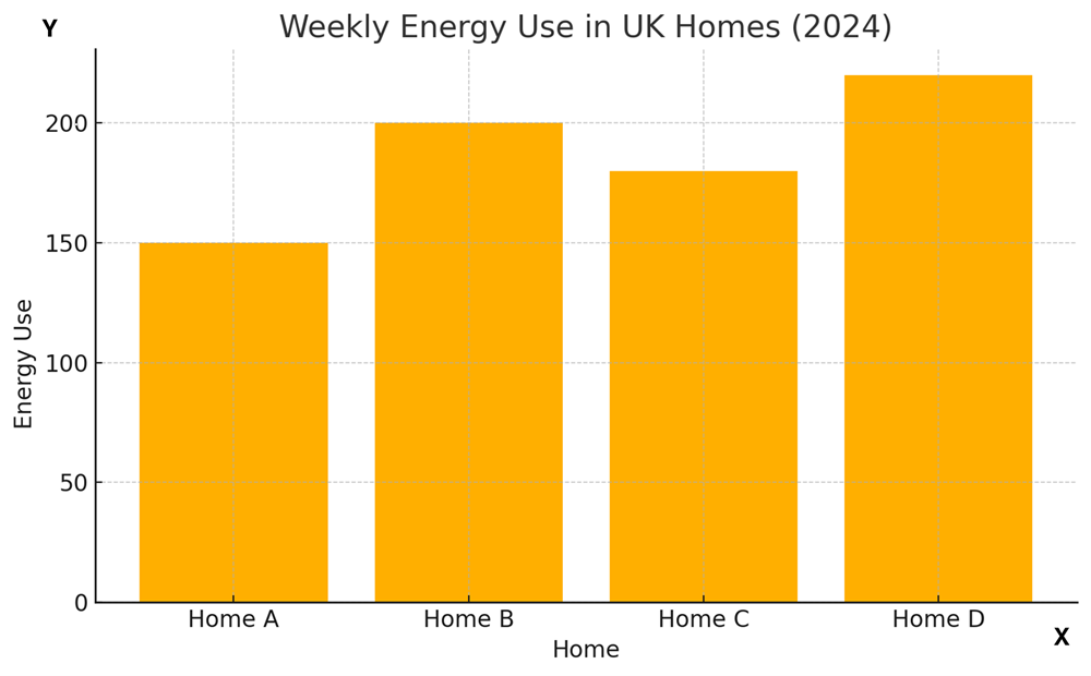
Data from: Weekly energy use table
| Home | Weekly energy use |
|---|---|
| A | 150 |
| B | 200 |
| C | 180 |
| D | 220 |
Which of these is the most likely unit on the vertical (y) axis?
- Pounds (£)
- Litres
- Kilowatt-hours (kWh)
- People
The correct answer is C Kilowatt-hours (kWh).
The chart is about energy use, and energy at home is commonly measured in kilowatt-hours (kWh).
Pounds would show cost, litres are used for liquids like water or fuel, and people wouldn’t be a measurement of energy.
3. Tables
Tables summarise and display precise information, such as numerical values, in rows and columns with appropriate headings. The structured format makes it easy to look up and compare information.
Let's look at some examples.
Class timetable
Let’s imagine you work as a learner support assistant and are expected to accompany a student to all their lessons. In the class timetable below, the column headings contain the days of the week (Mon to Fri), and the row headings show daily class times.
To check what class you should attend on a given day and time: locate the class time in the first column and then look along this row until you find the subject listed under the day (e.g. ‘Thu’) column heading.
| Mon | Tue | Wed | Thu | Fri | |
|---|---|---|---|---|---|
| 09:00 - 10:30 | Maths | English | Art | Geography | Languages |
| 10:40 - 12:10 | Physics | Geography | Maths | Languages | English |
| 12:10 - 13:00 | Lunch break | ||||
| 13:00 - 14:30 | Biology | Maths | English | History | Music |
| 14:40 - 16:00 | Languages | Art | History | English | Maths |
Data check
What time is the Music class on Friday?
The Music class runs from 13:00 to 14:30. You can find this by locating 'Music' in the column with the 'Fri' heading, and then looking along this row to find the row's heading (time slot) in the first column.
Daily sales report
In the daily sales report below, the number of teas and coffees sold in a cafe during the last week are listed. The column headings contain the type of coffee, or tea, and the row headings show the days of the week.
To check the number of sales in each category on a particular day: locate the day in the first column and then read the values under each of the column headings in this row.
| Americano | Latte | Flat white | Cappuccino | Tea | |
|---|---|---|---|---|---|
| Monday | 76 | 14 | 20 | 12 | 35 |
| Tuesday | 60 | 30 | 14 | 25 | 17 |
| Wednesday | 57 | 28 | 30 | 22 | 25 |
| Thursday | 37 | 32 | 12 | 27 | 14 |
| Friday | 70 | 36 | 18 | 32 | 28 |
| Saturday | 72 | 35 | 27 | 16 | 32 |
| Sunday | 55 | 25 | 23 | 27 | 40 |
Data check
How many lattes and flat whites were sold on Thursday?
32 lattes and 12 flat whites. Locate Thursday in column 1 and then moving along this row, note the figures in the 'Latte' and 'Flat white' columns.
The daily sales report table above gives precise information, however displaying the same data in a graph or chart could make it easier to spot trends, such as the most popular order, or the busiest day, as we'll see in the following pages.
Some tables include a total row at the bottom of one or more columns. This row adds up all the values in that column, giving you a quick overview of the total amount. Totals are useful for checking overall patterns or making comparisons.
The example below shows the number of participants from different regions signing up for activities and events at a business conference.
| Region | Keynote | Financial planning workshop |
AI strategy workshop |
Digital marketing workshop |
|---|---|---|---|---|
| Highland | 56 | 11 | 20 | 22 |
| Outer Hebrides | 31 | 3 | 9 | 19 |
| Orkney | 15 | 2 | 4 | 8 |
| TOTALS | 102 | 16 | 33 | 49 |
So, if we look at the column for the AI strategy workshop, we can see that there are 20 participants from Highland + 9 from Outer Hebrides + 4 from Orkney = a total of 33 participants signed up.
4. Charts and graphs
While tables provide precise information and values, they can be difficult to interpret at a glance.
Charts, graphs, and pictograms can be more immediately engaging, as they present a visual overview which can quickly help the viewer to:
- identify trends
- compare values
- understand proportions
- recognise patterns and outliers.
Charts summarise data in a simple, visual format, providing a snapshot of data highlights which can be understood by a general audience.
For example in the pie chart below, segment sizes can easily be compared, providing an immediate visual impression of a data set.
Graphs are often aimed at a specific audience, technical or scientific for example, allowing relationships between variables to be studied in more depth.
For example, an initial impression of the data plotted in the scatter chart below is not immediately revealing; it requires closer study.
In the following pages we will look at examples of the most common types of charts and graphs.
4.1. Pie chart
A pie chart is a circular chart, cut into segments, or slices. Each segment represents a proportion of the whole and can quickly demonstrate where there are wide differences between values.
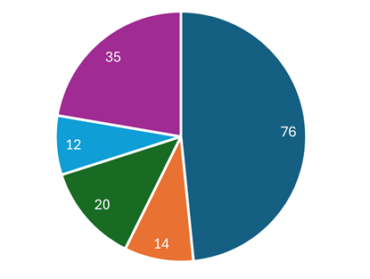
For example, in the pie chart below, we can instantly see that Americanos accounted for nearly half of all sales on Monday.
Data from: Daily sales table.
| Americano | Latte | Flat white | Cappuccino | Tea | |
|---|---|---|---|---|---|
| Monday | 76 | 14 | 20 | 12 | 35 |
| Tuesday | 60 | 30 | 14 | 25 | 17 |
| Wednesday | 57 | 28 | 30 | 22 | 25 |
| Thursday | 37 | 32 | 12 | 27 | 14 |
| Friday | 70 | 36 | 18 | 32 | 28 |
| Saturday | 72 | 35 | 27 | 16 | 32 |
| Sunday | 55 | 25 | 23 | 27 | 40 |
Although the visual impact of the different sized segments is perhaps the main reason you might choose a pie chart, data labels can also be included. In this example the data labels provide actual quantities sold for each category.

A pie chart provides visual impact for a snapshop of data. Another chart type would be more appropriate where access to multiple sets of data is required. For example, a pie chart could not show the breakdown of tea and coffee sales, for each day of the week, as we could do with a bar chart.
Data check
This chart shows the total numbers of each category sold during one week, with Americano being the clear favourite. Which category had the smallest number of sales?
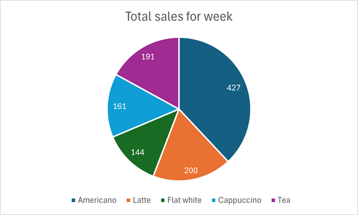
Flat whites were the least requested drink during this week: the number sold was 144.
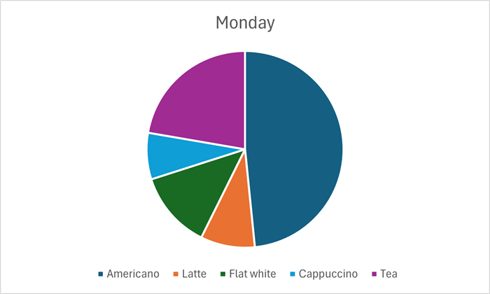
Data check
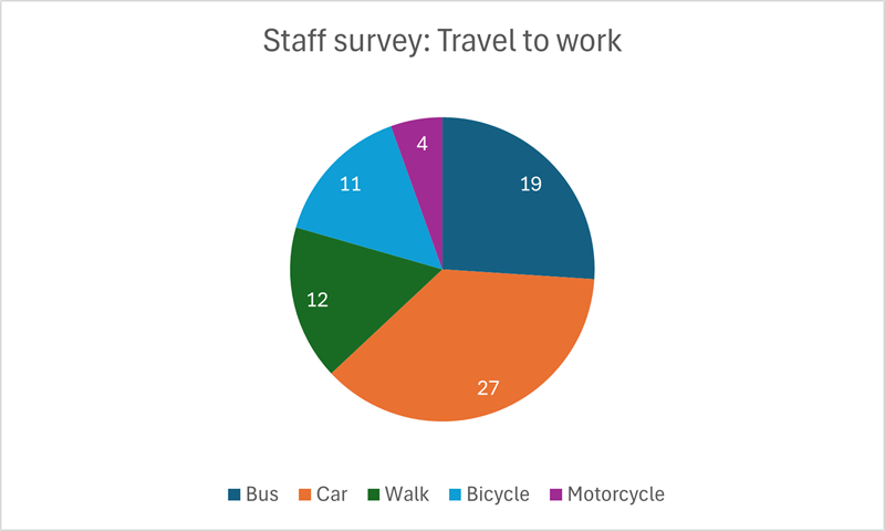
This pie chart shows the different travel to work methods used by staff working for a local business.
Data from: Staff travel table.
| Bus | Car | Walk | Bicycle | Motorcycle |
|---|---|---|---|---|
| 19 | 27 | 12 | 11 | 4 |
- What is the method of travel used by most staff?
- How many staff walk to work?
- How many staff in total were surveyed?
- Most of the staff (27) use a car to get to work.
- Twelve (12) members of staff walk to work.
- The total number of staff surveyed was 73. This is the sum of all the segment data labels.
4.2. Bar chart
Also known as a column chart, a bar chart represents data using vertical bars, which enable a quick comparison of values across different categories.
The categories are displayed horizontally along the bottom of the chart (the x axis), with a vertical value scale on the left (the y axis).
Data labels can be added to each vertical bar to provide exact figures, however keeping it simple, as in this example, gives an immediate picture of how things are.
A legend below the chart names the category represented by each colour.

Data from: Daily sales table.
| Americano | Latte | Flat white | Cappuccino | Tea | |
|---|---|---|---|---|---|
| Monday | 76 | 14 | 20 | 12 | 35 |
| Tuesday | 60 | 30 | 14 | 25 | 17 |
| Wednesday | 57 | 28 | 30 | 22 | 25 |
| Thursday | 37 | 32 | 12 | 27 | 14 |
| Friday | 70 | 36 | 18 | 32 | 28 |
| Saturday | 72 | 35 | 27 | 16 | 32 |
| Sunday | 55 | 25 | 23 | 27 | 40 |
Looking at the daily sales of coffee and tea from the previous page, for example, we can see at a glance that in this cafe, Americano is the most popular coffee.
Data check
What was the second most popular drink on Sunday?
Tea had the second highest volume of sales on Sunday, which in this case we can read as 40, because the bar touches the horizontal line representing this value. Other categories are not so easy to read and without data labels would have to be estimated, but we still have a quick visual representation for each, which is the main purpose of this chart.
Stacked column chart
A stacked column chart displays categories, over time, as part of a whole. The daily sales report in this format has one column for each day of the week, with the volume of sales for each category stacked within these.

Visually, we can still see that sales of Americano outstrip other options, but without data labels, totals for each have to be estimated. However, the stacked chart does show us that Friday had the highest sales in total, with sales on Saturday very slightly behind.
Data check
Which day had the least total sales?
Thursday had the least number of sales. The stacked bar reaches to slightly above the 120 sales mark.
4.3. Line graph
A line graph, or line chart, uses straight lines to connect data points, to show trends and relationships in data over time or categories.
This example shows data collected over a week, but a similar chart could be used to show trends over months or years.
A legend below the chart names the category represented by each colour.

Data from: Daily sales table.
| Americano | Latte | Flat white | Cappuccino | Tea | |
|---|---|---|---|---|---|
| Monday | 76 | 14 | 20 | 12 | 35 |
| Tuesday | 60 | 30 | 14 | 25 | 17 |
| Wednesday | 57 | 28 | 30 | 22 | 25 |
| Thursday | 37 | 32 | 12 | 27 | 14 |
| Friday | 70 | 36 | 18 | 32 | 28 |
| Saturday | 72 | 35 | 27 | 16 | 32 |
| Sunday | 55 | 25 | 23 | 27 | 40 |
Markers can be included to show the data values used to create the chart.
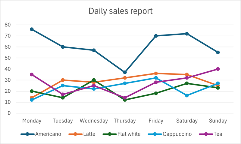
Multiple data series can appear very busy, making the trend information less of a focus. Line charts are most powerful, visually, when only one or two data sets are plotted.

Data check
Looking at the line chart (above) comparing sales of teas and Americanos, which day has the lowest sales of both?
Thursday has the lowest sales in both categories. For Americano, sales dip below 40, and tea sales are less than 20.
4.4. Area chart
An area chart is similar to a line chart, but highlights proportions by using colours, or shading, to fill the areas below the lines.
It can be difficult to discern individual values, however, particularly where areas overlap.

Data from: Daily sales table.
| Americano | Latte | Flat white | Cappuccino | Tea | |
|---|---|---|---|---|---|
| Monday | 76 | 14 | 20 | 12 | 35 |
| Tuesday | 60 | 30 | 14 | 25 | 17 |
| Wednesday | 57 | 28 | 30 | 22 | 25 |
| Thursday | 37 | 32 | 12 | 27 | 14 |
| Friday | 70 | 36 | 18 | 32 | 28 |
| Saturday | 72 | 35 | 27 | 16 | 32 |
| Sunday | 55 | 25 | 23 | 27 | 40 |
A stacked area chart reorders the categories to clearly show the proportion of each to the total value. However this reordering can cause confusion. For example the highest sales (Americano) in our Daily sales report appear at the bottom of the stack, with the lowest (teas) at the top of the stack, which may not seem logical.
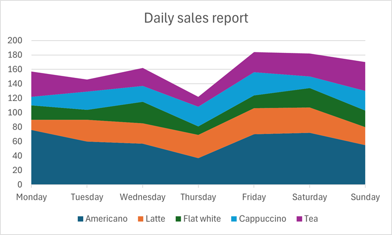
As with line charts, a simple area chart can be most useful when used to show relationships, and highlight differences, between one or two data sets
Looking at teas and Americanos only, from the Daily sales report, it is clear that sales of Americanos are at least double those of teas on most days.
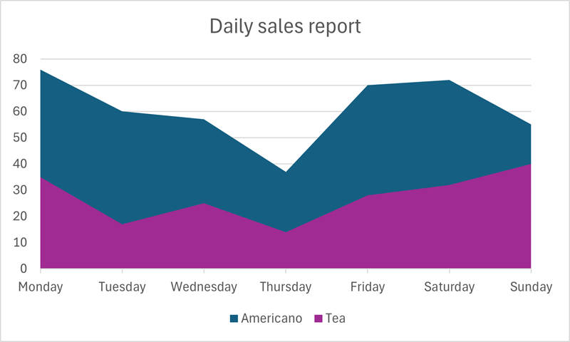
Data check
Looking at the chart above, on what day of the week do the number of teas sold reach a value greater than half of the number of Americanos sold?
On Sunday, the proportion of teas sold is clearly greater than half of the Americano sales. Americano sales are between 50 and 60 on the y axis, and teas are around 40.
4.5. Pictogram
A pictogram uses images, or symbols, to represent data in a simplified, visual format.
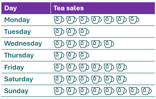
Each tea-cup represents 5 teas sold.
Data from: Daily sales table.
| Americano | Latte | Flat white | Cappuccino | Tea | |
|---|---|---|---|---|---|
| Monday | 76 | 14 | 20 | 12 | 35 |
| Tuesday | 60 | 30 | 14 | 25 | 17 |
| Wednesday | 57 | 28 | 30 | 22 | 25 |
| Thursday | 37 | 32 | 12 | 27 | 14 |
| Friday | 70 | 36 | 18 | 32 | 28 |
| Saturday | 72 | 35 | 27 | 16 | 32 |
| Sunday | 55 | 25 | 23 | 27 | 40 |
This pictogram shows tea sales for each day of the week, rounded to the nearest 5. There are 7 cup symbols alongside Monday, which indicates that 7 x 5 = 35 teas (to the nearest 5) were sold that day.
Data check
Looking at the pictogram, both Friday and Saturday have 6 cups. What were the approximate sales of teas on these days?
6 x 5 = 30, so approximately 30 teas were sold on both of these days.
A check of the data table shows that actual figures were (Friday) 28 and (Saturday) 32, however these have been rounded in order to represent an approximate sales picture using simple icons.
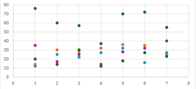
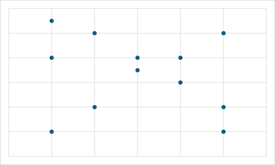
4.6. Scatter chart
Scatter charts plot the x, y coordinates of pairs of variables, providing a visual representation of the data which can be examined for potential relationships.
These charts are aimed at specific audiences - technical or academic for example - and can be difficult to interpret if not in those fields. This section, therefore, provides only a brief overview of the main features.
A scatter chart has been prepared using student test scores, alongside the number of tutorials each student attended. This chart will help the academic team to see if there is a link between the number of tutorials attended and the test results achieved.

Data from: Student Test Results table
| Student | Tutorials attended | Test result |
|---|---|---|
| A | 0 | 50 |
| B | 0 | 60 |
| C | 0 | 80 |
| D | 0 | 55 |
| E | 1 | 50 |
| F | 1 | 55 |
| G | 1 | 65 |
| H | 1 | 60 |
| I | 1 | 70 |
| J | 1 | 75 |
| K | 2 | 60 |
| L | 2 | 80 |
| M | 2 | 71 |
| N | 2 | 75 |
| O | 3 | 80 |
| P | 3 | 85 |
| Q | 3 | 75 |
| R | 3 | 78 |
| S | 4 | 80 |
| T | 4 | 85 |
| U | 4 | 90 |
| V | 5 | 95 |
| W | 5 | 90 |
| X | 5 | 85 |
| Y | 5 | 97 |
The scale on the x-axis (0 to 5), along the bottom of the chart, shows the the number of tutorials attended. The scale on the y-axis shows test scores achieved.
Looking at the chart, the test scores, on the whole, appear to rise with the number of tutorials taken. So we could say that the chart shows a positive relationship, or positive correlation.


Positive correlation
As one variable increases, the other also increases.

Negative correlation
As one variable increases, the other decreases.
No correlation
No relationship is apparent between the variables.