Use 'Print preview' to check the number of pages and printer settings.
Print functionality varies between browsers.
Printable page generated Monday, 6 May 2024, 7:31 PM
Processing and analysing AMR data
Introduction
This module looks at how antimicrobial resistance (AMR) data is transformed into information, locally, nationally and globally. It provides an overview of the stages from data collection, to data management and data analysis. It introduces the core concepts, approaches and methods for analysing data, including descriptive and inferential statistics, and how they can be used to answer important questions about AMR. Sources of error and bias will also be reviewed.
This module is part of a series of modules related to AMR data. You should complete Fundamentals of data for AMR and Sampling (either the animal health or human health version) in order to understand the basics of AMR data before starting this module. By the end of the module, you should be able to:
- describe components of the information cycle
- list and explain principles of best practice for data collection
- list and explain principles of best practice for data management
- explain the difference between descriptive and inferential statistics
- calculate measures of central tendency
- understand concepts related to hypothesis testing
- interpret reported findings from a hypothesis test, including strength of statistical evidence, and potential sources of error and bias.
Activity 1: Assessing your skills and knowledge
Rate each statement below on how confident you feel about each learning outcome. This activity is for you to reflect on your own knowledge and skills before completing the module (some of which you may have learned in previous modules).
Please use the following scale:
- 5 Very confident
- 4 Confident
- 3 Neither confident nor not confident
- 2 Not very confident
- 1 Not at all confident
1 Recap: data analysis principles
In the module Fundamentals of data for AMR, you learned about the basics of data for AMR, antimicrobial use (AMU) and antimicrobial consumption (AMC). The table below reminds you of the definitions of core terms that you will need for this module.
| Term | Definition |
|---|---|
| Data | Data are any observations or sets of observations or measurements that represent attributes about an entity, also referred to as a |
| Variable | A variable is an attribute used to characterise a data unit. They are called variables because their values can vary from one data unit to another and may change over time. Here are examples of commonly used variables:
Variables can be classified into numeric (quantitative) and categorical (qualitative) variables. Numeric variables can be further defined as either continuous or discrete, and categorical variables as either nominal or ordinal. |
| Dataset | A dataset is a collection of separate pieces of data that is treated as a single unit by a computer. Datasets often represent data in the form of a data table, in which columns represent variables and rows represent data values corresponding to each data unit. |
| Indicator | An indicator is a variable that has attributes directly relevant to decision-making. It is useful to determine whether, for example, the objectives of a program have been achieved, or a threshold for action has been reached. Most indicator variables are not directly observed and have to be calculated from the values of other variables. Given their importance in supporting decision making, indicator variables should have SMART characteristics (Specific, Measurable, Achievable, Attributable, Relevant, Realistic and Time-bound). |
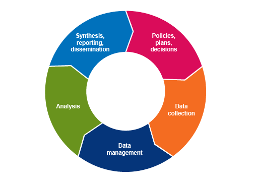
In the module Fundamentals of data for AMR, you were introduced to the ‘information cycle’ (Figure 1). It refers to the cyclical process of turning data into relevant, usable information that supports evidence-based decision making. In the Sampling modules, you learned about sources of AMR data and how representative samples of the population can be designed. In this module, you will learn about principles of best practice for collecting and managing AMR-related data, and how it can be analysed and interpreted. Other modules cover other aspects of the information cycle, for example, the modules Communicating AMR data and Using AMR data for policy making address the reporting, dissemination and use of AMR data.
2 Data collection best practice
Data collection (i.e. obtaining data from its source) involves making decisions about which data to collect. This includes sampling, which is covered in detail in the previous module, but also includes consideration of which data and variables to collect for each sampled unit. In this section, we will review principles of best practice for AMR data collection, which will ultimately maximise the usefulness and reliability of AMR data analysis.
Best practice for AMR data collection (or, indeed, for any data collection) is a set of principles that ensure that data, and the process by which they are collected, are:
- beneficial for users
- standardised
- repeatable
- relevant
- timely
- disaggregated.
2.1 Beneficial for users
Data collection processes need to be designed for
Who is a data collector, and who is a data provider?
- A data collector is a person whose job is to plan, manage and implement the entry of data into databases. They are not necessarily involved in generating the data themselves. For example, a data collector might be employed to review and enter data from hospital records into an AMR database or to conduct a survey about AMU in hospitals.
- A data provider is a person or organisation that generates and submits relevant data as part of their day-to-day work. For example, doctors who prescribe antibiotics using electronic prescribing software that automatically stores these data in a database are providers of data about AMU and, therefore, data providers.
When data collection processes are not straightforward for data collectors and providers, two main risks are that the data collectors or providers will either not submit data regularly (or on time) or enter poor quality data. If they do not perceive that collecting and providing good quality data will lead to good quality information (and therefore outcomes) that benefits them, they may not be motivated to invest time and effort into providing good data. The burden on and benefits for data collectors and providers should be a primary consideration when designing data collection systems.
Activity 2: Generating and using AMR data in your workplace
Reflect on AMR, AMU and/or AMC data collection occurring in your workplace:
- What type(s) of AMR and AMU or AMC data are collected?
- Who collects or provides these data? Are you a data collector or provider?
- What benefits do you think these data collectors and providers obtain from this activity? Does it inform their day-to-day work, for example? If you are a data collector or provider, reflect on your own experience.
- What challenges or problems do these data collectors or providers encounter from collecting AMR, AMU or AMC data? If you are a data collector or provider, reflect on your own experience.
Answer
The answers you gave to these questions will depend on your particular workplace and your role within it. However, even if you are not directly involved in collecting or providing AMR, AMU or AMC data, you need to be aware of how it is done and of the challenges the processes pose to those involved.
2.2 Standardised
Data must be collected in a standardised fashion. This means that variables need to have a similar meaning across different contexts. This means careful consideration of the measurement unit or classification:
Numeric (quantitative) data should be recorded along with the measurement unit (for example, if the variable is ‘body weight’, is it recorded in kilograms or in pounds?).Categorical (qualitative) data should be recorded using standardised, freely available and widely accepted classification schemes whenever possible. For example, diagnoses may be recorded using the latest version of the International Classification of Diseases (ICD). More information on ICD can be found here.
Electronic data collection is the best way to enable standardisation of collected data. Electronic data capture ideally allows each event (e.g. prescription of antimicrobial medicine) to be entered in the system only once, reduces the rates of error associated with data entry and allows for immediate validation of the data values with the primary data provider. When the data are collected manually and entered later in a data management system, it is usually not possible to go back to the primary data provider to verify data that appear incorrect. Manual entry is also time consuming and less efficient as the data are entered more than once (for instance, first on a paper form and second in a spreadsheet). However, this may not be avoidable in some circumstances where only paper-based data collection methods are available.
Consider some examples of data checking that can be built into electronic data collection systems:
- Automated date validation at submission ensures an accurate log of data entry records is maintained. This also prevents errors such as dates in the future or a date from the past that isn’t possible (such as a patient’s date of birth in the year 1850 instead of 1950).
- The data entry tool can be used to set plausible minimum and maximum values for a given variable, for example, setting patient weight in kilograms to have a maximum value of (say) 550kg. If a user enters a value such as 620kg, the system will automatically detect an error and request that the value is checked or corrected before the data entry is finalised.
Activity 3: AMR data collection in your workplace
Reflect on the following questions.
How are AMR, AMU or AMC data collected in your workplace?
- Are they captured electronically or in paper-based format?
- Are there measures in place to standardise data in your workplace? For example, are there forms where you must tick a box rather than writing your own response? How does this achieve standardisation?
2.3 Repeatable
Repeatable data collection means that for a study population, two or more different individuals would collect the same data if using the same approach/method (allowing for small differences due to random error). The data collection process should be designed to minimise the amount of subjectivity and interpretation left to the data collector. Repeatability is in part linked with standardisation, as clear definitions of the data to be collected will allow the same results to be collected by different observers.
For example, the World Health Organization (WHO) provides a standardised methodology called a
- Is a patient who was discharged at lunchtime on the day of the survey eligible for inclusion?
- If a patient is admitted half an hour after the survey starts, should they be included?
To address this, the WHO specifies that for the purpose of a PPS, an inpatient is defined as a patient who has been admitted to a hospital ward at or before 8 a.m. on the day of the survey. Applying this definition means that there is less room for interpretation of the methodology by the data collector, and hence the data collection process is more repeatable.
Inevitably, there will always be some inherent variability and uncertainty in measurements of data, which is related to random error or bias. This means that repeatability may not always be achieved. For example, the temperature of a patient taken by a nurse at the time of sample collection may be different from the temperature taken by the same nurse, at the same time, with a different thermometer. Recording additional metadata, such as the method used for measuring temperature, may help to understand the variability when analysing and interpreting the data.
2.4 Relevant
Data should be collected with the aim of answering specific questions, as data collection is never a goal in itself. An example of a relevant and specific question for which we might collect data is ‘what proportion of antimicrobials given to cattle are used for growth promotion?’. Other relevant goals are to establish baseline values or to measure progress achieved towards an objective. Irrelevant data collection is a waste of resources and will cause disengagement amongst stakeholders.
In the case of AMR data, this involves collecting the variables that will contribute towards understanding patterns of resistance, but avoiding the collection of unnecessary data. For example, when taking samples from people for the purpose of monitoring AMR, relevant data may include whether the person is healthy or unwell, and if they are unwell, what the primary diagnosis is and where it was made (e.g. hospital or community-based care). Irrelevant data might include their marital status, health insurance status and use of medications for hypertension (high blood pressure) – these data are commonly collected by health practitioners, but they don’t help us to understand AMR specifically.
2.5 Timely
Where possible, data capture (entering collected data into an electronic system) should be in real-time. First, this allows for informed decision making to reflect current trends observed in the data. Second, this allows timely feedback to be given to the data providers, and therefore increases the benefits they might derive from data submission and the likelihood of them contributing meaningful, complete data to the system.
2.6 Disaggregated
Last, data should be collected and stored at the highest possible resolution and never aggregated (summarised into a group or class) in the database. Any aggregation for analysis or presentation should come at a later stage. For example, when disc diffusion is used to assess antimicrobial sensitivity of a bacterial strain, the inhibition zone diameter should be recorded as a quantitative, raw value in the database. The classification as resistant or susceptible may then be derived from the recorded diameters, on the basis of the accepted cut-off values (taken from international standards such as the European Committee on Microbial Susceptibility Testing, EUCAST or the Clinical Laboratory Standards Institute, CLSI). Should these cut-off values change, you can then review the raw data and update if necessary. This is not possible if only aggregated data (for example, only that classification of ‘resistant’ or ‘susceptible’) is recorded.
3 Data management best practice
- It provides a single validated source of information.
- It protects privacy and confidentiality.
- It is secure.
- It is adaptive and responsive.

3.1 Providing a single source of validated information
A good data management system comprises a single data repository. Independent data managers oversee the infrastructure, and governance groups determine policies and practices relating to functionality, access and use of the system. Data may be submitted using multiple means, but should be integrated, stored, analysed and presented in one system. For example, data should not be managed using multiple spreadsheets stored in different locations. In this case, the absence of a single repository means that multiple versions of the same data may be available, with no way for the user to know which one is the most accurate and up to date.
This does not mean that back-up versions cannot be created and stored. This is a different process, and such back-ups are named and flagged as back-ups: they will never be changed, updated or modified, unless the primary repository is lost and a back-up is restored in its place.
3.2 Protecting privacy and confidentiality
Data should remain as disaggregated as possible, but with measures to ensure that privacy and confidentiality are maintained. Privacy and confidentiality can be maintained by de-identifying the data (e.g. removing names, phone numbers and street addresses from the main database) and implementing a permission system that controls access to the data. For example, a doctor may have access to confidential information including names and contact details. By contrast, the data analyst or hospital administrator may only have access to the patient numeric identifier (
3.3 Ensuring data security
Governance and ethical requirements will also provide guidance on how data should be stored securely. For health-related data, data security measures should be put in place that ensure that only authorised users can access data. These measures will vary depending on the data management system used. For example, when data are collected in spreadsheets, this includes measures such as password protection, restricted access to computers where the data are stored. For electronic information systems, more advanced measures are put in place, which require the guidance of experts in the domain. Data should also be automatically backed up in multiple locations, to allow recovery of as much data as possible in case of loss of or damages to the primary data repository.
3.4 Adaptive and responsive
Data management systems need to be flexible and responsive to changing needs and circumstances. Inflexible systems become outdated quickly, often failing to integrate with other systems effectively. Adaptable systems can change when priorities and requirements change; this is especially relevant in animal and public health surveillance, where priority concerns are constantly evolving. Related to this, a good data management system will have a database design that promotes interoperability with other information systems.
There are few good examples (yet) of adaptive and responsive designs for AMR surveillance anywhere in the world. To get an idea of what such a system could look like, Box 1 summarises how the US Centers for Disease Control (CDC) is developing a syndromic surveillance system that can be readily adapted to detect and respond to new health threats, which could include a new type of AMR. However, such systems are not yet available in many countries.
Box 1: Overview of US CDC syndromic surveillance system
Putting data to work: from signal to response
Using data from emergency departments nationwide to track symptoms has become a model for electronic data exchange between health care and public health. CDC’s National Syndromic Surveillance Program helps connect local, state, and national public health agencies to data from more than 4,000 healthcare facilities in 45 states, and Washington, DC. Officials can unite nationwide and act quickly when something unusual happens. They can also monitor how well their response is working and adjust as needed.
Enhancing syndromic surveillance and linking multiple data sources is one focus area of CDC’s strategy to improve surveillance data.
- Newer: Cloud-based technology and analysis tools allow local and state users to visualise and share information from an increasing number of health facilities.
- Faster: Near-real-time data allows users to quickly detect and monitor health impacts in their local communities and across the country.
- Smarter: As new health threats emerge, such as Zika infections and opioid overdoses, syndrome definitions can be quickly developed and standardised.
- Better: As new analytic methods are added and participation increases, data sources can be expanded and integrated with other systems, including electronic death records.
3.5 Reflecting on data management best practice
Now that you’ve reached the end of this section, try the following activity.
Activity 4: AMR data management in your workplace
Reflect on how AMR data is managed in your workplace by assessing how confident you are that the data management system meets these best practice recommendations. Take some notes reflecting on your answers.
- Our data management system is centralised:
- Confident
- Unsure
- Not confident
- Our data management system protects privacy and confidentiality:
- Confident
- Unsure
- Not confident
- Our data management system is secure:
- Confident
- Unsure
- Not confident
- Our data management system is adaptive and responsive:
- Confident
- Unsure
- Not confident
4 Data analysis for AMR
Data analysis is about identifying and summarising meaningful patterns in data that are of value to stakeholders. Descriptive analysis is the process of summarising data, while inferential statistics allow the user to investigate relationships between variables and assess whether there is evidence that one variable (an
4.1 Recap: measuring AMR
In the module Fundamentals of data for AMR, you learned that AMR is generally measured using the following three indicators:
- Proportion of specimens where a target pathogen was isolated: This relates to the frequency with which pathogens are isolated from human or animal specimens. When sampling healthy food animals, for example, not all animals will have the target pathogen of interest (such as Salmonella spp.).
- Proportion of
isolates that were resistant to each antimicrobial: This is a commonly used indicator in human and animal AMR surveillance. - Distribution of minimum inhibitory concentration (MIC): Results from broth/agar dilution testing are often presented as distributions of MICs for particular isolates and antimicrobials.
Assuming high quality data collection, these indicators meet most of the key principles of best practice listed above with the exception of generating direct benefits to those who provide or collect data (Table 2). For example, if the proportion of isolates resistant to each antimicrobial is only summarised at national level, and this data is only reported several months after it was originally collected, this may not be very helpful for clinicians to understand the best way to prevent or treat resistant infections in their patients. When designing AMR surveillance systems, particular emphasis should be given to the data providers’ needs and perceptions to ensure long-term submission of quality data.
| Best practice principle | Indicator | ||
|---|---|---|---|
| Proportion of specimens with target pathogen isolated | Proportion of isolates resistant | Distribution of minimum inhibitory concentrations Footnotes a | |
| Standardised | ✓ | Usually Footnotes b | ✓ |
| Repeatable | ✓ | ✓ | ✓ |
| Generate benefit for users | Depends | Depends | Depends |
| Measurable | ✓ | ✓ | ✓ |
| Relevant | Unlikely to inform action | ✓ | ✓ |
Footnotes
Footnotes aEquivalently, the distribution of growth inhibition zone diameters when the disc diffusion method is used. Back to main textFootnotes
Footnotes bStandardised cut-off values for resistant isolates are available but they are not systematically used by all laboratories and over time. Back to main text4.2 Descriptive analysis
Descriptive analyses are conducted for three key purposes:
- to detect errors and clean data
- to understand the distribution of the data and the relationships between variables
- to generate hypotheses.
They are generally the first step in any data analysis and consist of characterising and visualising the dataset of interest. In this section, we will look at how to describe a variable depending on its type and how to describe the relationship between two or more variables. Aspects related to data visualisation will be covered in more detail in the module Summarising and presenting data.
4.2.1 Descriptive statistics for categorical variables
For example, let us consider the variable ‘resistance to levofloxacin’. This variable was measured for 120 methicillin-resistant Staphylococcus aureus (MRSA) isolates. This variable has two levels: ‘resistant’ for 38 of the isolates and ‘susceptible’ for the others. Descriptive statistics for this variable can be reported in a single sentence of text:
- As a count: AST results showed that 38 of the 120 MRSA isolates were resistant to levofloxacin.
- As a proportion: the AST results showed that 31.7% of the 120 MRSA isolates were resistant to levofloxacin (i.e. ((38/120)*100)).
Below is an example of reporting descriptive statistics in sentence form from the literature. This sentence reports relative frequencies (as percentages) for four variables containing the resistance status (resistant/susceptible) for four antimicrobials.
“A large number of MRSA isolates showed resistance to levofloxacin (83.9%), ciprofloxacin (83%), erythromycin (77.7%) and clindamycin (72.3%).” (Kot et al., 2020)
In the examples above, the outcome variable had only two levels (resistant/susceptible), and tabular or graphical representation would not provide much more additional information. When categorical variables have more than two levels, or when multiple variables with two levels are presented in parallel, they may also be displayed in a frequency table (Table 3) or in a graphical format using a bar chart (see module Summarising and presenting AMR data). When presenting proportions, it is good practice to also provide the corresponding counts, or frequencies, especially in cases where small sample sizes are used. The example in Table 3 shows the breed of cattle from which a target organism was recovered. The categorical variable ‘breed’ has four levels: Jersey, Guernsey, Holstein Friesian and Unknown.
| Breed | Frequency | Relative frequency (%) |
|---|---|---|
| Jersey | 234 | 20.7 |
| Guernsey | 63 | 5.6 |
| Holstein Friesian | 800 | 70.7 |
| Unknown | 34 | 3.0 |
| Total | 1131 | 100 |
4.2.2 Descriptive statistics for a numeric variable
Descriptive statistics for numeric variables (continuous or discrete) include measures of
Measures of central tendency include:
- The
arithmetic mean : the sum of all values divided by the number of values, also known as the ‘average’. The arithmetic mean provides a valid measure of the central tendency only when the data is approximatelynormally distributed . This method is the most often used to estimate means, and therefore when someone reports a ‘mean’ or ‘average’ without specifying which type of mean, it is an arithmetic mean by convention. - The
geometric mean : the nth root of the product (multiplication) of the values, where n is the number of values. This measure is often used to summarise MIC values, which are generally not normally distributed. - The
median : the middle value in an ordered set of values. The median is the best measure of central tendency to use for non-normal data, for example,skewed orbimodal data. - The
mode : the most common value in a set of values. It can only be calculated when there are repeated values.
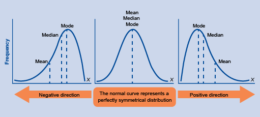
When data are normally distributed, the mean, median and mode are equal to each other. When the data are not normally distributed, each of these measures can take different values (Figure 2). Which measure is most useful therefore depends on the distribution of the data and the analysis objectives.
Activity 5: Calculating measures of central tendency
The ages of the first 12 patients diagnosed with MRSA during a hospital survey were 55, 98, 64, 81, 1, 70, 43, 29, 79, 84, 87 and 64. Calculate the (arithmetic) mean, median and mode of these ages.
Answer
The mean age is 63 (to the nearest integer) – the sum of the ages (755) divided by 12; the median is 67 – in the ordered set of ages the 6th and 7th ages are 64 and 67 and so, since there are an even number of ages, the median is the mean of these central ages (64 and 70); and the mode is 64, which occurs twice. As this distribution is skewed towards older ages, the median is higher than the mean.
Measures of dispersion include:
- The
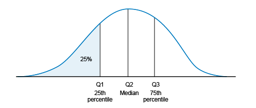
range : this is the difference between the minimum and maximum observed values. Percentiles : percentiles are calculated by ordering the set of values and dividing it in parts of equal sizes (with the same number of values inside). Commonly used percentiles are quartiles, as shown in Figure 3: the first quartile (Q1, also known as the 25th percentile) is the median of the lower half of the ordered dataset (25% of the values are below Q1). The second quartile (Q2) is the median. The third quartile (Q3) is the median of the upper half of the ordered dataset (75% of the values are below Q3).- The
interquartile range : this is the difference between the Q3 and Q1 values. - The
variance : this is a measure of how far on average each value in the set of values is from the mean. It is calculated as the average of the squared differences from each data point to the mean value. - The standard deviation: this is the square root of the variance, and therefore also measures how spread out the data is from the mean. Unlike the variance, the standard deviation is in the same unit of measurement as the data itself, which means it is easier to compare directly to the mean value.
These descriptive statistics may be reported in text, displayed in tables (see example in Table 4) or graphically (histograms and box-and-whisker plots, for example, which will be covered in the module Summarising and presenting AMR data).
| Minimum | 3 |
|---|---|
| Q1 | 12 |
| Median | 29 |
| Mean | 19 |
| Q3 | 75 |
| Max | 267 |
Feeling confused? It’s probably been a while since you learned about these concepts in high school. If you would like a refresher, you can watch the two videos below for worked examples of measures of central tendency (video 1), and for a refresher and worked examples on measures of dispersion (video 2).
Transcript: Video 1 8.5 minutes
Summary transcript of video 1: Video explaining the three common measures of central tendency and how they are determined: the mean (or arithmetic mean) as the sum of the values of the data points divided by their number; the median as the middle data point when the data points are arranged in numerical order; and the mode as the most common value. Each of these is valuable in different circumstances, although the mean is most frequently used.
Transcript: Video 2 12.5 minutes
Summary transcript of video 2: Video explaining measures of dispersion of a dataset, and how these can distinguish between very different datasets that nevertheless have the same mean. These include the range (the overall spread of the dataset); the variance (the average of the squares of the differences between each data point and the mean); and the standard deviation as the square root of the variance.
4.2.3 Joint descriptive statistics for two or more variables
The descriptive statistics presented above were applied to the variables of interest separately, for demonstration purposes. This rarely happens in practice – instead, two or more variables are generally jointly presented to assess the type of relationship between them.
Such relationships are generally considered between one variable as the
- The relationship between one categorical variable and one (or more) categorical variable(s) can be displayed in a contingency table or cross-tabulation. An example contingency table for jointly describing two or more variables is shown in this separate PDF file.
- The relationship between one numeric variable and one (or more) categorical variable(s) can be displayed in a summary table, as shown in Figure 4, or graphically (see module Summarising and presenting data).
- Last, the relationship between a numeric variable and another numeric variable can be displayed graphically (if it is inconvenient to display such variables in a table).
Activity 6: Identifying exposure and outcome variables
Activity 7: Interpreting exposure and outcome variables
4.3 Inferential statistics
4.3.1 Null hypothesis testing
Null hypothesis testing is a formal statistical approach to evaluating evidence for two different interpretations of a relationship between two variables, the null hypothesis and
The null hypothesis (H0) is generally that there is no difference between two groups. For example, the prevalence of resistant isolates in the group which received antimicrobial treatments is the same as the prevalence in the group which did not. The alternative hypothesis (Ha) is that there is a difference, that is, in this example that the prevalence of resistant isolates differs significantly between these two groups.
To reject or retain the null hypothesis, we need to assume a statistical model which represents our scientific hypothesis and then collect the data. Then, we calculate the probability of observing data as extreme as the data in hand, should the null hypothesis be true; this is the
4.3.2 Statistical errors, confidence and power
Type I error (whose probability is commonly noted as α) is where our findings reject the null hypothesis (no difference) when in fact it is true. In other words, a false positive. By convention, the threshold for α is usually set at 5%, implying it is acceptable to have a 5% chance of rejecting the null hypothesis when it is true. Type II error (whose probability is commonly noted as β) is where our findings uphold the null hypothesis when it is not true. In other words, a false negative. By convention, the threshold for β is usually set at about 20%. The difference in probabilities of a false negative and a false positive relates to the burden of evidence required to reject the null hypothesis. For example, it is more important to exclude false positives when making claims such as one treatment being better than another (if that is not true), than to exclude false negatives such as there is no difference between two treatments (even when there is).
By contrast, the two other cells in Table 5 illustrate when correct inferences are made: accepting the null hypothesis when it is true or rejecting it when false. Confidence (1-α) is the probability of retaining the null hypothesis when it is true. In this case, we are accepting that the observed difference in the data is due to chance only.
| Truth | |||
|---|---|---|---|
| H0 true | H0 false | ||
| Our findings | H0 true | Correct (1-α) | Type II error (β) |
| H0 false | Type I error (α) | Correct (1-β) | |
Hint: Does this sound familiar? If you’ve completed one of the Sampling modules, you were introduced to the concepts of confidence and power. Now, you can see that confidence level, which is usually set as 95%, is 1 – α, and power, which is usually set at 80%, is 1 – β.
4.3.3 Confidence intervals
For example, zoom in on the first row of data in the separate PDF file: the best estimate of the percentage of community isolates resistant to ampicillin in 2009 is 39.6%, but the 95% CI is 36.3%–43.1%. This means that if this study was to be repeated a very large number of times, we would expect the percentage of isolates resistant to ampicillin to fall in this range (36.3%–43.1%) 95% of the time.
4.3.4 Limitations of null hypothesis testing
Basing inferences solely on whether a probability (i.e. p-value) exceeds an arbitrary cut-off is not good practice. Other elements must be considered, such as the strength of association and the sample size used. In a setting where we are assessing the difference between two means, for example, the strength of association can be assessed by calculating the difference between or the ratio of these two means. While the p-value tells us whether this difference is statistically significant, the value of this difference tells us whether it is a clinically or biologically important effect. For example, let us consider that the proportion of isolates resistant to erythromycin in a given selection of patients decreased from 10.0% to 9.8% after applying a set of recommendations for combating AMR in a hospital for one year. After accounting for sample sizes, the difference is statistically significant. But is a decrease of 0.2% meaningful? If you would be the funder of this intervention, would you consider that a successful outcome?
Although p-values are widely used throughout the scientific literature, they are commonly misinterpreted. Many scientists and statisticians are now advocating abandoning the use of p-values altogether. In practical terms, the use of an arbitrary cut-off (e.g. 0.05) means that for p=0.045 we will consider that the observed difference is ‘significant’, while this would not be the case for p=0.055. It is not so straightforward in reality, and statistical tests provide information in terms of strength of evidence for or against a given hypothesis rather than a binary answer. It is more useful to think about p=0.001 as providing stronger evidence for an effect than either p=0.04 or p=0.06. There are a range of advanced alternative approaches to null hypothesis tests, which report and interpret p-values in different ways. The key thing to remember is to always interpret the strength of the statistical evidence alongside consideration of how clinically or biologically important the effect is.
4.3.5 Choosing statistical tests (OPTIONAL)
This section is optional in that it provides more detail on the statistical tests that can be applied to analyse the data. If you have time and/or such analysis is important to the type of work you do, you should study this section.
Many different statistical tests have been developed, and we will only look at the most common ones in this module. Firstly, statistical tests can be classified as
We will look at two categories of tests in this section. First, let us consider the tests to use when the exposure variable is a categorical variable. In this case, statistical tests allow us to assess differences between counts or means of the outcome variable at different levels of the exposure variable (e.g. assess the differences in average healing time (outcome variable) for different treatments A, B and C). The choice of such a statistical test depends on the type and characteristics of the data being analysed. One way to determine what test is most appropriate is to identify the type of outcome variable, the number of groups being compared (i.e. in our example – there are three levels of the variable ‘treatment’: A, B and C) and whether the assumptions for the test are met (this step may be informed by the descriptive analysis). Table 6 lists the most important assumptions for each test. For example, a non-parametric Mann-Whitney test might be used to test whether there are differences in the presence of AMR genes in bacterial isolates sampled from patients in hospitals, compared to patients in the community.
Statistical tests in a second category are those used when the exposure variable is numeric. In this case, tests allow users to assess the existence of a significant relationship between the (numeric) outcome and exposure variables. When there are no other variables to consider, such a test is called a correlation or collinearity test. The most commonly used correlation tests are Pearson’s r (parametric, normally distributed variables) and Spearman’s ρ rank correlation (non-parametric). For example, researchers conducting a multi-country study have data on the prevalence of resistance to a particular antimicrobial for two target organisms for 20 countries. If they want to know whether resistance to a particular antimicrobial in one target organism is related (correlated) to resistance in the second target organism, they could use a test for correlation. If additional variables need to be considered in the analysis, multivariable regression models can be constructed, though this is beyond the scope of this module.
Table 6 provides an overview of the types of statistical tests you can conduct according to the type of data you have. If you’re just starting out in learning statistics, some of this information might seem very complex, but you don’t need to understand it all now. Keep a copy of this table for future reference for when you plan and conduct your own analyses of AMR data. An important point to note for now is that results obtained from statistical tests are only valid when all the assumptions for the test are met. This important point is not always easy to assess in practice. Two important assumptions common to the seven tests presented in Table 6 are that the observations are based on a random sample and that they are independent from each other. When observations are not independent, for example, when several observations are obtained from the same individual at different points in time (repeated observations) or from a matched study design, then other tests should be used, such as paired sample t-test or mixed-effect regression models. Such tests are out of the scope of this course.
| Parametric or non-parametric? | Outcome variable | Number of groups Footnotes 1 | Statistical test | Key assumptions |
|---|---|---|---|---|
| Parametric | Categorical: nominal with two levels (dichotomous) | Two or more | Chi-squared test | Expected frequency in any cell of a contingency table is not |
| Non-parametric | Categorical: ordinal, or numeric when assumptions for a t-test are not met | Two groups | Mann-Whitney U test (Wilcoxon rank-sum test) |
|
| Non-parametric | Categorical: ordinal, or numeric when ANOVA test assumptions are not met | Three or more groups | Kruskal-Wallis test | Outcome can be ranked |
| Parametric | Numeric | Two groups | Student’s t-test |
|
| Parametric | Numeric | Two or more groups | One-way ANOVA |
|
| Parametric | Numeric | Two or more groups | Simple linear regression with one exposure variable |
|
| Parametric | Categorical: nominal with two levels (dichotomous) | Two groups | Binomial logistic regression | Linear relationship between the exposure and log odds |
Footnotes
Footnotes 1This is the number of groups being compared i.e. the number of levels in the exposure variable. Back to main text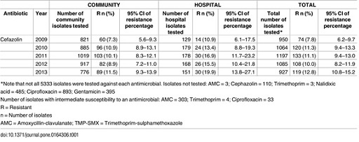
Activity 8: Conducting a statistical test
- Draw a simplified two-by-two contingency table with only the count values that are of interest for the first part of this activity (comparing 2009 with 2010) from the data presented in Figure 5.
Hint: the contingency table should show the number of isolates with were identified as resistant and the number identified as susceptible in each year, in all settings.
Answer
| Isolate status | Year 2009 | Year 2010 |
|---|---|---|
| Resistant | 74 | 120 |
| Susceptible | 876 | 944 |
The number of susceptible isolates each year was obtained by removing the number of resistant isolates from the total number tested, i.e. 950 and 1064 isolates in 2009 and 2010, respectively.
- Using an online calculator for carrying out Chi-squared tests (such as this one), use the data above to perform a Chi-squared test.
Hint: if you made your table in Excel, just copy and paste into the calculator. Alternatively, you can enter the data by copying and pasting the text below:
| Isolate status | Year_2009 | Year_2010 |
|---|---|---|
| Resistant | 74 | 120 |
| Susceptible | 876 | 944 |
Answer
The p-value obtained from the test is 0.010, indicating that there is a statistically significant difference between the proportion of resistant isolates in 2009 and in 2010. Note that the result also presents the Chi-squared statistic (which is 6.62) and degree of freedom (which is one) – these parameters are used to calculate the p-value, but apart from recognising that Chi-squared tests are suitable for data where the outcome variable is categorical (Table 6), you don’t need to understand more about these parameters in this module.
- Do the same test to compare the proportion of resistant isolates between 2010 and 2011.
Answer
The Chi-squared statistic for this second comparison is 0.003, with one degree of freedom. The p-value obtained from the test is 0.95, indicating that there is no evidence for a statistically significant difference between the proportion of resistant isolates in 2010 and in 2011.
5 Recap: bias and error in AMR data
Once we have conducted a null hypothesis test, we now have more information about the importance of the finding. But this isn’t the only piece of information we need to consider when interpreting the result. Sources of error and bias in AMR studies and surveillance programs (described in the module Fundamentals of Data for AMR) include:
random error systematic bias (orsystematic error )- selection bias
- information bias (including misclassification error, recall bias and observer bias)
confounding .
For a refresher, check the glossary for the definitions of these terms.
Hypothesis testing allows us to address random error. However, other types of error and bias may still affect the inference (conclusions) drawn from the data. Systematic bias should be accounted for when interpreting findings, as the analysis cannot correct for it. Lastly, although there is no test for confounding, it can be accounted for by using multivariable statistical modelling, which is outside the scope of this course.
Activity 9: Interpreting the results of data analyses
6 Strengthening AMR data analysis locally and globally
AMR surveillance programs are often focused on generating and reporting descriptive statistics, which is valuable given the lack of available knowledge in many species and contexts. However, there are several steps that we can take as a global AMR community to improve the quality of information we have to combat the threat of AMR. Inferential data analysis plays a key role in this context. It is also important to focus on assessing the impact of factors that we can control, given that AMR is also influenced by factors that we cannot readily change. For example, there is ongoing research to identify the duration of antimicrobial treatment that optimises individual patient or animal outcomes whilst minimising the risk of AMR. This research will inform recommendations on optimising antimicrobial course length for both doctors and veterinarians.
Another area of active research is the link between AMU in animals and AMR in humans. This is relevant for improving antimicrobial stewardship programmes in agriculture and understanding how and when a decline in antimicrobial use in agriculture would be expected to lead to a decline in AMR in pathogens carried by humans. Finally, there are ongoing efforts to manage AMR better worldwide through establishment of effective, standardised global protocols for analysis of AMR data. Current efforts include GLASS and the OIE’s global monitoring of AMU in animals. Global efforts also focus on creating ways for AMR data to more directly benefit users (such as patients, farmers, clinicians and veterinarians), as this is key to support long-term, high-quality data collection.
7 End-of-module quiz
Well done – you have reached the end of this module and can now do the quiz to test your learning.
This quiz is an opportunity for you to reflect on what you have learned rather than a test, and you can revisit it as many times as you like.
Open the quiz in a new tab or window by holding down ‘Ctrl’ (or ‘Cmd’ on a Mac) when you click on the link.
8 Summary
In this module, you have been introduced to the basics of data collection, data management and data analysis, including descriptive and inferential analyses.
You have seen that data collection and management are two key stages of the information cycle, as they determine the quality of AMR data. Without following best practice in these areas, we would not be able to work with reliable data, and therefore any data analysis effort would be of limited use. You have learned the key statistics used to summarise categorical and numeric variables and some of the possible applications to AMR data analysis. Last, you have been introduced to the basics of statistics for AMR data analysis.
You should now be able to:
- describe components of the information cycle
- list and explain principles of best practice for data collection
- list and explain principles of best practice for data management
- explain the difference between descriptive and inferential statistics
- calculate measures of central tendency
- understand concepts related to hypothesis testing
- interpret reported findings from a hypothesis test, including strength of statistical evidence, and potential sources of error and bias.
Now that you have completed this module, consider the following questions:
- What is the single most important lesson that you have taken away from this module?
- How relevant is it to your work?
- Can you suggest ways in which this new knowledge can benefit your practice?
When you have reflected on these, go to your reflective blog and note down your thoughts.
Activity 10: Reflecting on your progress
Rate each statement below on how confident you feel about it now that you have completed the module.
Please use the following scale:
- 5 Very confident
- 4 Confident
- 3 Neither confident nor not confident
- 2 Not very confident
- 1 Not at all confident
When you have reflected on your answers and your progress on this module, go to your reflective blog and note down your thoughts.
9 Your experience of this module
Now that you have completed this module, take a few moments to reflect on your experience of working through it. Please complete a survey to tell us about your reflections. Your responses will allow us to gauge how useful you have found this module and how effectively you have engaged with the content. We will also use your feedback on this pathway to better inform the design of future online experiences for our learners.
Many thanks for your help.
References
Acknowledgements
This free course was collaboratively written by Melanie Bannister-Tyrrell, Anne Myers and Clare Sansom, and reviewed by Siddharth Mookerjee, Claire Gordon, Natalie Moyen, Peter Taylor and Hilary MacQueen.
Except for third party materials and otherwise stated (see terms and conditions), this content is made available under a Creative Commons Attribution-NonCommercial-ShareAlike 4.0 Licence.
The material acknowledged below is Proprietary and used under licence (not subject to Creative Commons Licence). Grateful acknowledgement is made to the following sources for permission to reproduce material in this free course:
Images
Module image: Sebastien Decoret/123RF.
Figure 1: Ausvet Pty Ltd.
Section 3 (laptop): photo by Lukas Blazek/Unsplash.
Figure 2: publisher unknown.
Figure 3: Han, J. et al. (2012) Chapter 2, ‘Getting to know your data’ in the Morgan Kaufmann series in data management systems, Data Mining, 3rd edn, Morgan Kaufmann, pp. 39–82, https://doi.org/ 10.1016/ B978-0-12-381479-1.00002-2.
Figures 4 and 5: Anderson, D.J., Kaye, K.S., Chen, L.F., Schmader, K.E., Choi, Y., Sloane, R., et al. (2009) ‘Clinical and financial outcomes due to methicillin resistant Staphylococcus aureus surgical siteiInfection: a multi-center matched outcomes study’, PLoS ONE, 4(12): e8305, https://doi.org/ 10.1371/ journal.pone.0008305 – this file is licensed under a Creative Commons Attribution 3.0 Unported (CC BY 3.0) licence, https://creativecommons.org/ licenses/ by/ 3.0/.
Tables
Tables 2–6: Ausvet Pty Ltd.
Text
Section 4.2.3: Fasugba, O., Mitchell, B.G., Mnatzaganian, G., Das, A., Collignon P, Gardner, A. (2016) ‘Five-year antimicrobial resistance patterns of urinary Escherichia coli at an Australian tertiary hospital: time series analyses of prevalence data’, PLoS ONE, 11(10): e0164306, https://doi.org/ 10.1371/ journal.pone.0164306 – this file is licensed under a Creative Commons Attribution 4.0 International (CC BY 4.0) licence, https://creativecommons.org/licenses/by/4.0/.
Every effort has been made to contact copyright owners. If any have been inadvertently overlooked, the publishers will be pleased to make the necessary arrangements at the first opportunity.