Week 8: Communicating with data
Use 'Print preview' to check the number of pages and printer settings.
Print functionality varies between browsers.
Printable page generated Monday, 6 April 2026, 3:29 AM
Week 8: Communicating with data
Introduction
At the end of last week you looked at one way of communicating with data, the use of tables. This week this theme will be continued by taking a look at graphs and charts. These give us a means of displaying data visually, and as the saying goes, ‘a picture paints a thousand words’! So, graphs and charts can be a very useful way of presenting data clearly and at the same time showing any possible patterns. You’ll be considering how to present and interpret graphs and charts, as well as the care that needs to be taken when doing this to ensure that you are really being presented with the full picture.
In the following video Maria introduces Week 8, the final week of the course, and the final quiz for your badge:

Transcript
After this week’s study, you should be able to:
- read and construct line graphs to display information
- read and construct bar charts to display information
- read and construct pie charts to display information
- critically interpret graphs and charts.
1 Graphs and charts
At the end of last week you looked at how useful tables are for summarising a lot of data concisely, clearly and accurately. However, sometimes you want to get an overall message across quickly and this may well stay hidden in a table of data. In this situation you can use a graph or a chart instead. Graphs can also be used to explore relationships between sets of data, such as the way in which a sunflower grows over a season.
You have probably seen different types of graphs and charts in your day-to-day life, such as when watching the TV, reading a newspaper or on the internet. Here is a flavour of some you may have encountered.
Bar charts
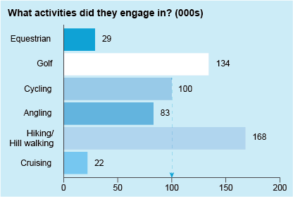
These allow a visual comparison between different categories. For instance, in Figure 1 you can see very quickly that the hiking/hill walking category was the most popular activity, and cruising the least popular.
Pie charts
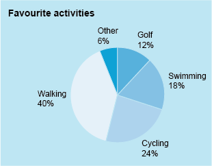
Again, these allow a quick visual comparison between categories but this time using percentages rather than the actual data. This pie chart shows very clearly that walking is the favourite activity.
Line graphs
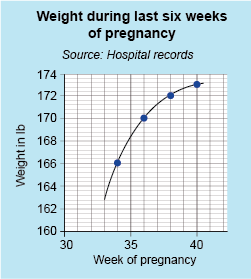
Finally, a line graph, where all the plotted points are joined, can show clear relationships between the plotted data. In this case, the curve shows that the weight (or as it’s properly known, mass!) of a woman increases over the last six weeks of her pregnancy, but that this weight gain slows towards the end. This is shown by the flattening out of the curve in Figure 3.
You may well have come across other charts or graphs, but as these are three of the most common types, bar and pie charts and line graphs will be the focus of this week. To get you started, in the next section you will look at plotting points on a line graph.
2 Line graphs
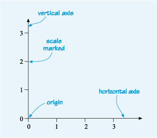
Line graphs are constructed by plotting points on a grid. Figure 4 shows two lines at right angles to each other that set up a grid. These are called the horizontal axis and the vertical axis. Each axis is marked with a scale, in this case from 0 to 3. The point where the two axes meet and where the value on both scales is zero is known as the origin. (Note: ‘axes’ is the plural form of ‘axis’.) This is not only the basis for all line graphs, but also for bar charts.
In Figure 5, the horizontal axis has been labelled with an ‘x’ and the vertical axis with a ‘y’. This is because the horizontal axis is usually known as the x-axis and the vertical axis as the y-axis.
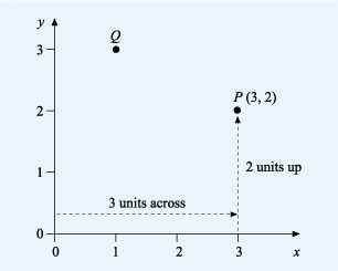
The location of any point on the grid by its horizontal and vertical distance from the origin. These are always shown with the horizontal distance first and in the form (x,y), where x and y are the respective distances from the origin to the point. This is known as the coordinates of the point. The horizontal distance being the x-coordinate and the vertical distance the y-coordinate.
Look at point P in Figure 5. To get to point P from the origin, you move three units across and two units up. Alternatively you can say that point P is opposite 3 on the x-axis and 2 on the y-axis. This gives us the coordinates for P of as (3,2), with an x-coordinate of 3 and a y-coordinate of 2.
In the same way, point Q is one unit across and three units up, so Q has coordinates (1, 3).
coordinates do not need to be positive numbers though. You’ll see in the next section how both the x and y axes can be extended to include negative numbers, just as a number line can.
2.1 Negative coordinates
Figure 6 shows the axes extended downward and to the left, to include negative values. The coordinates of the plotted points still have the same configuration, that is, x first, followed by y, and are read in the same way as before. For example, point B is three units to the left of the origin, so its x-coordinate is –3. It is one unit up, so its y-coordinate is 1. So B has coordinates (–3, 1).
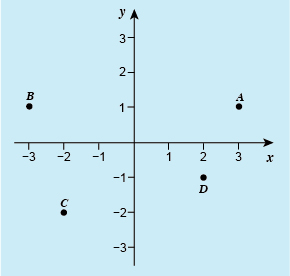
Now it is your turn to try your hand at reading the remaining coordinates from Figure 6 in this first activity of the week.
Activity 1 Reading coordinates
Write down the coordinates of points A, C, and D, shown in Figure 6. What are the coordinates of the origin?
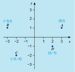
Answer
A is opposite 3 on the x-axis, so its x-coordinate is 3. It is opposite 1 on the y-axis, so its y-coordinate is 1. The coordinates of A are (3, 1).
C is opposite -2 on the x-axis, so its x-coordinate is -2. It is also opposite -2 on the y-axis, so its y-coordinate is also -2. The coordinates of C are therefore (-2, -2).
The coordinates of D are (2, -1).
The origin has coordinates (0, 0).
As well as being able to read coordinates of points on a graph it is also important to be able to plot them yourself, for when you need to draw your own line graph. There is probably not much need for this in your day-to-day life, but many different study areas make use of graphs to show data and relationships. So a good working knowledge of how to construct a graph will stand you in good stead if you continue with your studies in the future.
You’ll look at plotting points in the next section.
2.2 Plotting points
Plotting points is essentially the same as reading the coordinates of a point. This means going along the x-axis to the given coordinate, and then vertically upwards until you are opposite the correct place on the y-axis. The point can then be marked with one of three symbols: a dot, as in the examples here, a cross, or a dot with a circle around it. This last option just makes the plotted point clearer if the points are joined with a line.
The next activity will give you some practice at plotting points. It would be useful to do this exercise on graph paper because it is much easier to plot the points accurately if you have a grid to work with. Fortunately, you don’t have to rush out and buy lots of graph paper because you can print out as much as you need, if you have a printer.
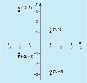
Activity 2 Plotting points
Draw x- and y-axes, with a scale on these from -3 to 3. Mark the points E at (1, 1), F at (–2, –1), G at (1, –3) and H at (–2, 3).
In the examples so far, all the coordinates were whole numbers and the scales were also marked at whole unit intervals. As with a number line though, there is nothing to stop us also showing fractions of whole units. Let’s take a look at this now.
2.3 Decimal coordinates
Marking a scale with fractions of whole units allows us to plot points using decimal coordinates such as (1.8, –2.1).
In Figure 9 below, each unit along the axes has been divided into ten, so each grey line represents a tenth of a whole unit, or 0.1. Point A has the coordinates (1.3, 0.8), as it is plotted 1.3 units across to the right of the origin and 0.8 units up.
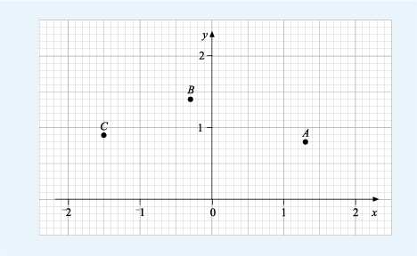
Now, we’ve done the first point for you, complete the coordinates for the other points shown in the next activity.
Activity 3 Reading decimal coordinates
Write down the coordinates for the points B and C on the graph above.
Answer
B is plotted at the point which is 3 intervals to the left of the origin on the horizontal scale and 4 intervals past the 1 mark on the vertical scale, i.e. opposite -0.3 on the x-axis and opposite 1.4 on the y-axis. So the coordinates of B are (-0.3, 1.4)
Similarly, the coordinates of C are (-1.5, 0.9).
2.4 Displaying data on a graph or chart
You have seen that, provided you have both an x- and a y-coordinate, you can plot a point on a chart. So if a set of data consists of pairs of data values, then that data can be plotted on a graph. This enables patterns between the data to be assessed visually, as well as mathematically. This is for future study though!
There are several steps to take when drawing a graph, which can be summarised as follows:
- Choose an appropriate scale for both axes.
- Label both axes, including a brief description of the data and the units.
- Give your graph a suitable title.
- State the source of data.
- Plot the points accurately.
- Join the plotted points with a line or smooth curve if appropriate.
Following these steps will ensure that any graph is clear, easy to read and well presented.
Let’s look at one of these steps in more detail now – choosing the scales.
2.5 Choosing the scales for a graph or chart
Choosing appropriate scales can take more time than other elements of constructing a graph. They can need careful consideration, as they affect the whole look of the graph. Scales are usually chosen to illustrate the data clearly, making good use of the graph paper and using a scale that is easy to interpret.
In the examples considered so far, the scales on both axes were the same and both started at zero. However, this is not always appropriate. You’re going to investigate this using the example of a nurse monitoring the weight of a woman during the last few weeks of her pregnancy. The woman’s weight each week has been recorded as shown in Table 1 below.
| Week of pregnancy | 34 | 36 | 38 | 40 |
|---|---|---|---|---|
| Weight in kg | 75.6 | 77.4 | 78.1 | 78.5 |
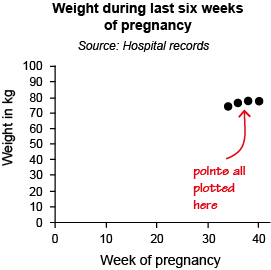
You could start both scales at 0, but then all the points would be plotted in the top right-hand corner, making the graph difficult to read, as can be seen in Figure 10 below.
Since the data on the x-axis start at 34 and finish at 40, a better scale on the x-axis would be one starting at 30 and ending at 42. Similarly, since the data for the y-axis are from about 75 to around 79, a scale on the y-axis that starts at 72 and ends at 79 would seem sensible. Using these scales, the points would be plotted as shown in Figure 11.
Hopefully you can see by comparing the two graphs that the second attempt, as well as being much clearer, just looks better! That is always a good test of how well a graph has been constructed.
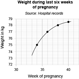
Note that as well as the scales being marked on the axes, these are labelled to show what is being measured, and in what units. The graph also has a title and source of data.
The points have been joined with a smooth curve as, in this case, you would expect the woman’s weight to change steadily between hospital visits over the period. So, it is reasonable to join the points to show the overall pattern or trend.
So, the graph has all the required elements.
If you have access to some graph paper, have a go at drawing your own graph in this next activity.
Activity 4 Drawing a graph
The data shown in Table 2 are the circumferences and diameters of various circular objects. All measurements are in centimetres.
| Diameter/cm | Circumference/cm |
|---|---|
| 4.4 | 14.1 |
| 6.6 | 20.9 |
| 8.6 | 27.0 |
| 10.3 | 32.3 |
| 23.0 | 72.8 |
(a) Construct a graph to show this data, with the diameter on the horizontal (x) axis and the circumference on the vertical (y) axis. Draw a straight line through the points.
Answer
(a) Your graph should look like this:
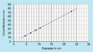
Note the title and labelling of the axes. You may have used a different scale from us if you had different graph paper. This is fine, as long as it makes best use of the paper and is easy to read from.
Finally in this section on line graphs you’re going to take a look at how to read from, and use, a graph.
2.6 Using a graph
As well as providing a visual representation of data, a graph can be used to infer more information than the data that you started with.
Look again at the change in weight of a woman during the last six weeks of pregnancy. Since you would expect the woman’s weight to change steadily between hospital visits, it is possible to use the graph to estimate her weight at other times during the six weeks.
For example, to estimate her weight at 35 weeks, first find 35 on the horizontal axis. Then from this point, draw a line parallel to the vertical axis, until the line meets the curve at point P. From P, draw a line horizontally, to meet the vertical axis. Read off this value: in Figure 13, it is about 76.2 kg.
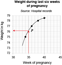
Determining values between the plotted points is known as interpolation.
Activity 5 Reading a value from a graph
Use the graph above to answer the following.
It may be helpful to print this page with the graph, so that you can draw lines on the graphs to identify values. You may also use an object with a straight edge, such as a ruler or piece of paper, and hold it up to your monitor to help you visualise where certain points appear in relation to the axis.
- a.What is the woman’s weight at 37 weeks?
Answer
a.Find 37 on the horizontal axis and draw a line vertically up to the curve. Then draw a line horizontally from this point to intersect the vertical axis. This value is approximately 77.6 kg.
The woman’s weight at 37 weeks is estimated to be about 77.6 kg.
- b.When do you think the woman’s weight was 76 kg?
Answer
b.Find 76 kg on the vertical axis. Draw a horizontal line to meet the curve. Then draw a line vertically down to meet the horizontal axis. Read off the value: it is just below 35 weeks.
So the woman’s weight is estimated to have been 76 kg in week 34.
As well as inferring other data from the graph in some cases it is possible to estimate the coordinates of points that lie outside those plotted. This is known as extrapolation. However, you must be confident that the graph continues in a similar manner so you do need to be cautious: you cannot be certain that patterns shown in graphs will continue.
For instance, in our example it would not be sensible to extrapolate beyond 40 weeks, as this is the usual length of a normal pregnancy.
The graph can also be used to determine the overall trend in the data — that is, how one value is changing with the other. In this case, the graph shows that the woman gained weight quite rapidly between weeks 34 and 36, but from week 36 to week 40 she gained less.
So, careful use of a line graph can prove a very powerful tool when investigating collected data.
The next section looks at bar charts and the different ways these can be drawn, depending on the data that you have and what you want to show.
3 Bar charts
Last week, you saw data from Fáilte Ireland presented in tables. On their website they also illustrate other data in the form of bar charts, as shown in Figure 14 below. This represents the numbers of visitors participating in different activities.
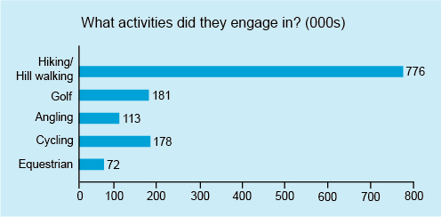
In a bar chart, the length of each bar represents the number in that category. Because the bars on this chart are horizontal, the chart is known as a horizontal bar chart. However, bar charts can also be drawn with vertical bars. Note that each bar has the same width, and since the bars represent different and unrelated categories, the bars do not touch each other and are separated by gaps.
The authors of this chart have made it easy to read as they’ve marked the values represented by each bar directly on the chart. If the values had not been marked on the bars, they could have been estimated by drawing a line from the end of the bar and seeing where it intersected the horizontal axis, just as you did with the line graph.
So, rather than spending time on reading from a bar chart let’s move on to constructing one.
3.1 Drawing a bar chart
The same basic guidelines apply to drawing a bar chart as they do to drawing a line graph. There are a few differences though. So, the steps to follow are:
- Choose an appropriate scale for both axes.
- Label both axes, including a brief description of the data and any units.
- Give your graph a suitable title.
- State the source of data.
- Draw the bars for each category accurately.
Use the skills that you have already gained when drawing a line graph to complete this activity.
Activity 6 Drawing a bar chart
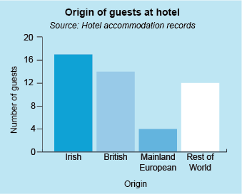
Last week you created the following table showing information about hotel guests:
| Nationality | Child | Adult | Senior | Total |
|---|---|---|---|---|
| Irish | 8 | 5 | 4 | 17 |
| British | 4 | 6 | 4 | 14 |
| Mainland European | 0 | 3 | 1 | 4 |
| Rest of the world | 6 | 4 | 2 | 12 |
| Total | 18 | 18 | 11 | 47 |
Use the table to draw a vertical bar chart that shows the total number of guests in each of the nationality categories. Mark the nationality categories on the horizontal axis and the number of guests on the vertical axis.
Another way of showing data on a bar chart is using a component bar chart, which can give more detail than the basic examples that have already been looked at. This will be the subject of the next section.
3.2 Component bar charts
In our last example of the quantity of guests from different nationalities in a hotel, you could add extra detail by showing how these totals were broken down into the different age groups. To do this you can split each bar into three different sections, where the length of each section represents the number of guests in that age group. The resulting bar chart would then be a component bar chart, as shown in Figure 16. Notice that a key (or ‘legend’) has been added to the graph to explain the shading for the different age categories.
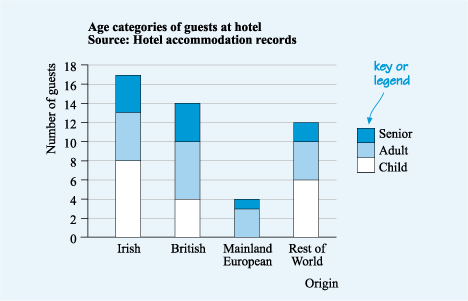
When you read a component bar chart, you need to find the height of the relevant section to determine the quantity that it represents. For instance, the top of the section representing British adults is opposite the 10 on the vertical scale. The bottom of that section is opposite the 4. Thus, the number of British adults is the difference between the top and the bottom of the section, which is 6.
Another type chart is called a comparative bar chart. This again shows more detail than a standard bar chart, but in a different way to a component one, as you’ll see now.
3.3 Comparative bar charts
A comparative bar chart places bars representing sections from the same category adjacent to each other. This allows for a quick visual comparison of the data.
For example, another way of categorising the data that you have been working with so far would be to split each nationality into the number of females and males. The resulting comparative bar chart would be as shown in Figure 17.
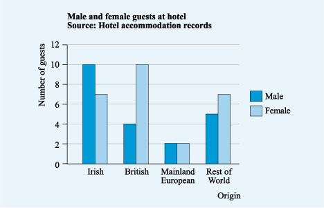
It is easy to see why this is called a comparative bar chart, as it is straightforward to compare the data – for example it is easy tell that many more visitors from Britain were female.
Finally in this section on bar charts, notice how all these charts followed the same format, with the title and source clearly labelled and the axes and scales clearly marked, but they emphasised different aspects of the data. The first showed the totals from each nation, whilst the latter two gave more detail on this data. So when you are displaying data in a graphical form, it is important to choose a chart or graph that stresses the main points as simply as possible so that your reader can understand your chart quickly and easily.
Now it’s time to look at our final type of chart, the pie chart.
4 Pie charts
Although bar charts are useful to display numbers and percentages, sometimes you might want to stress how different components contribute to the whole. Pie charts are often used when you want to compare different proportions in the data set. The area of each slice (or sector) of the pie chart represents the proportion in that particular category.
For example, the pie chart in Figure 18 illustrates the favourite type of exercise for a group of people:
This pie chart shows the percentages for each category, so you can read these off directly. Even without the percentages marked, it would be clear that walking was the most popular activity overall as a proportion of the whole group.
Sometimes, however, the percentages are not marked on the chart, so the proportions then have to be roughly estimated by eye. This, of course, is not ideal for all situations when accurate data is required!
The next activity gives you a chance to practise reading a pie chart.
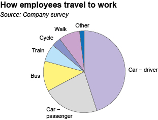
Activity 7 How employees travel to work
The pie chart in Figure 19 illustrates how employees in a particular company travel to work:
Use Figure 19 to answer the following questions:
(a) Do more people travel to work by bus or by train?
Answer
(a) The slice of the pie representing bus travel is larger than the slice representing train travel, so yes, more people travel by bus than by train.
(b) Would it be correct to say that the number of employees who travel to work as car drivers is about twice the number who travel as car passengers?
Answer
(b) The slice of the pie chart representing car drivers is about twice the size of the slice representing car passengers, so it is correct to say that the number of employees who travel to work as car drivers is about twice the number who travel as car passengers.
(c) Estimate the proportion of employees who travel to work by car, either as the driver or as a passenger.
Answer
(c) The two slices for car drivers and passengers cover about two-thirds of the circle, so about two-thirds of employees travel to work by car, either as the driver or as a passenger.
If necessary – and providing the pie chart has been drawn accurately – you can also work out the percentages by measuring the angle at the centre of the pie for each sector using a protractor. For example, the angle at the centre of the circle for the ‘Car passenger’ category in Activity 7 is about 80º.
Because a complete circle measures 360º, the fraction that this sector represents is , or 22%. So approximately 22% of the employees travel to work as car passengers.
However, as pie charts are often used to give an overall impression rather than detailed information, on many occasions a rough estimate will suffice.
This concludes our look at three different ways of displaying data visually. Before moving on to the last badged quiz for this course though, there are some words of caution for you on reading graphs.
5 Reading a graph with caution
The graph in Figure 20 below shows the monthly heating bills of a house before and after loft insulation was installed.
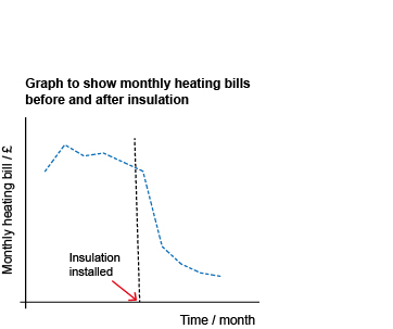
You should have noticed that there are important pieces of information missing from this graph that you now know should always be included.
The first is the source of the data. Without this you have no idea how the data were collected or how reliable the information may be. Was just one house used in the survey, or were many houses used?
The next, and this makes the graph almost meaningless, is that neither axes have any scales marked.
Suppose the scale on the vertical axis was from £50 to £51; if it was, the apparent drop in the bill after insulation would be negligible. However, if the scale went from £0 to £50, the drop might be of more interest.
What about the horizontal axis? You don’t know what time of year the data were collected or over what period. In fact, the data was collected from November to September, so the horizontal scale should have indicated this.
The graph appears to show a large drop in the heating bills after insulation was installed. However, without the scale on the vertical axis, it is impossible to say what kind of drop this is.
From the data you know that the drop in the monthly heating cost occurred in the May bill, just as the weather was warming up for the summer. So that means the reduced bills could simply be due to less heating being used in the summer.
So, overall, no conclusions can be drawn from this graph about the effectiveness of the insulation.
This illustrates an important point: when you are comparing two sets of data: you need to compare like with like. You would expect the bills for the summer to be less than those in the winter anyway, regardless of the presence or absence of loft insulation. It would be more appropriate to consider the amount of energy used for heating over two periods with similar weather.
So, although graphs and charts are very useful, it is important to read them critically, checking that all the information you need to interpret them is provided.
Another important point to note is that if the graph appears to show an association between two quantities, it does not prove that one has caused the other. For example, suppose the number of students in a town registering in a maths course rose from year to year and the number of burglaries in the town also rose – does this mean that the maths students have committed the burglaries? No, of course not! Both rises may be linked to some other factor, such as the number of people who have recently moved into the town.
6 This week's quiz
Well done, you’ve not only come to the end of this week’s study but you have also completed the final week in Succeed with maths – Part 2!
Go to:
Remember, this quiz counts towards your badge. If you're not successful the first time you can attempt the quiz again in 24 hours.
Open the quiz in a new tab or window (by holding ctrl [or cmd on a Mac] when you click the link).
7 Summary
After studying this week you should now be able to:
- read and construct line graphs to display information
- read and construct bar charts to display information
- read and construct pie charts to display information
- critically interpret graphs and charts.
So … congratulations on making it to the end of this week and Succeed with maths – Part 2! The subjects that you have studied, including measurement, patterns and formulas and working with data, have all laid the foundations of important areas of not only mathematical study but also many other areas. Maths is a fundamental tool for any scientist, economist, engineer, nurse or teacher, to name just a few. But, importantly, having a good grasp of these fundamentals will help you in your everyday life no matter what you do. So, as well as the personal achievement of completing the course, remember your new skills can help you every day as well as maybe opening new doors for you.
Every success with your onward journey, wherever this might lead.
If you’ve gained your badge you’ll receive an email to notify you. You can view and manage your badges in My OpenLearn within 24 hours of completing all the criteria to gain a badge.
You can now return to the course progress page.
Tell us what you think
Now you've come to the end of the course, we would appreciate a few minutes of your time to complete this short end-of-course survey (you may have already completed this survey at the end of Week 4). We’d like to find out a bit about your experience of studying the course and what you plan to do next. We will use this information to provide better online experiences for all our learners and to share our findings with others. Participation will be completely confidential and we will not pass on your details to others.
References
Acknowledgements
This course was written by Hilary Holmes and Maria Townsend.
Except for third party materials and otherwise stated (see FAQs), this content is made available under a Creative Commons Attribution-NonCommercial-ShareAlike 4.0 Licence.
Every effort has been made to contact copyright owners. If any have been inadvertently overlooked, the publishers will be pleased to make the necessary arrangements at the first opportunity.
Don't miss out:
1. Join over 200,000 students, currently studying with The Open University – http://www.open.ac.uk/
2. Enjoyed this? Find out more about this topic or browse all our free course materials on OpenLearn – http://www.open.edu/ openlearn/ free-courses/
3. Outside the UK? We have students in over a hundred countries studying online qualifications – http://www.openuniversity.edu/ – including an MBA at our triple accredited Business School.