Sampling (human health)

Introduction

To generate data on AMR in surveillance programmes or research studies, we first need to make decisions about how, where and from which entities (individuals or groups) to collect data. This is known as ‘sampling’.

This module will focus on sampling for AMR surveillance in human health, but will also draw comparisons to animal health, where relevant, to emphasise the importance of One Health approaches in tackling AMR.

After completing this module, you will be able to:

• describe the purpose of sampling individuals for AMR surveillance
• explain what factors need to be considered when choosing which individuals to sample for AMR surveillance
• recognise the lists of priority pathogens suggested for sampling in individuals
• list the steps involved in sampling individuals for AMR surveillance
• explain the common problems associated with identifying sampling frames and how they can be addressed.

1 Sampling basics

In this section we consider the basics of sampling: why and how to do it.

1.1 Why do we need to sample?

Have you ever taken part in a census, such as a national human population census? A census involves collecting data from every single unit (such as a human, animal, farm) in the population. Conducting a true census is a very resource-intensive activity. What happens if we would like to answer a question such as:

Is it necessary to collect data on every single inpatient in a country to answer this question? In most cases, it is impractical to conduct a census, especially when we need to collect specimens, such as blood, urine or faecal samples, from every single person in a population.

Fortunately, for the majority of research or surveillance, it is not necessary to conduct a census. Instead, we can select an appropriate sample of subjects from the population. Sampling allows us to make inferences about a larger population. But we can’t just pick any people we happen to find and expect that this ‘sample’ allows us to make inferences (apply the findings) to the entire population; instead, there are several steps we have to go through to ensure that our sample is representative (accurately reflects the characteristics) of the broader population that we are interested in. Going through these steps is the focus of this section.

1.2 Sampling terminology

How can we determine what constitutes an ‘appropriate’ sample? It is helpful to introduce some terminology as we go through the steps in selecting a sample.

Figure 1 From populations to samples.

First, we need to identify the population in which we are interested – this is known as the ‘target (reference) population’. Then we need to identify how we can choose a sample that is representative of the target population. There are three stages of defining the sample:

• source (study) population
• study sample
• sampling unit.

1.3 Sampling and validity

Why is it important to describe and identify these sampling parameters?

Here, we need to think about the ‘validity’ of sampling: how well a measurement represents the true situation. If you have already completed the Fundamentals of data for AMR module, you may recall that the concepts of external validity and internal validity were introduced. These concepts are defined in terms of the relationship between the study sample and the target population.

Figure 2 External and internal validity.

Show description|Hide description

A schematic diagram showing a source population as a subset of the target population, and a study sample as a subset of the source population. External validity represents the extent to which the source population can be extrapolated to the target population, and internal validity the extent to which the study sample represents the source population.

Figure 2 External and internal validity.

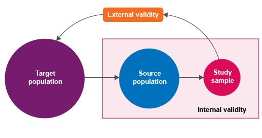
Epidemiological principles of sampling in animal populations are the same as the principles applied to sampling in human populations. In animal health, it is similarly necessary to define the target population, the source population, the study sample and the sampling unit. In animal health, a flock, herd or other group might be the lowest-level sampling unit: this is because in a herd, all the animals are in the same physical area and exposed to identical risk factors. By comparison, an individual is the most common lowest-level sampling unit in human health.

Activity 3 has an example of this.

2 Sampling frames

We now know that in order to sample from a population, we need to first identify the target population and the source (study) population. We then select the study sample. But how do we identify sampling units that form part of the source population? We need a sampling frame.

A sampling frame might be a list of all of the hospitals in the province(s) selected as the source population, along with a list of all the patients being treated at these hospitals (either as inpatients resident in hospital or outpatients attending walk-in clinics, depending on the topic of interest) in a defined time period. Note that because sampling frames include identifying information such as names and addresses, extra attention must be paid to ensuring that this information is stored and accessed securely by authorised members of the research team or surveillance programme (see the Legal and ethical considerations in AMR data module).

Because sampling frames constitute a data-collection process, they are subject to the same risks of error and bias as all other AMR-related data collection and analysis (see the Fundamentals of data for AMR module for more information on error and bias). Most of the time, available sampling frames do not perfectly correspond to the actual source population: for example, a sampling frame for AMR surveillance might consist of a list of all antimicrobial susceptibility tests (ASTs) performed in laboratories on samples collected from hospitalised patients in a city. However, not all patients with resistant infections are sampled, or the sample may not be fully tested – that is, may not be tested against all the drugs of interest. Some hospitals have limited capacity and experience with collecting samples for bacterial isolation and AST. Some patients may decline to have their sample tested if they have to pay a fee for the laboratory test. In general, a sampling frame should include facilities, such as hospital sites, that account for at least 80% of the target population.

In reality, sampling frames are not always available or complete, and therefore might not include all units in the source population, and so by extension are not representative of the target population. Examples include when there is a mix of public and private health facilities in an area, but only the public facilities are included in the sampling frame because it is more convenient to do so. For studies or surveillance of AMR or antimicrobial use (AMU) in the community, in many settings there is no complete list of every person who lives in a village or district of interest. This can make it difficult to collate a comprehensive list of sampling units to include in the sampling frame.

Three potential solutions to achieving representative sampling when no adequate sampling frame exists are summarised below:

• Random geographic coordinates sampling: An online tool generates a series of randomly selected map coordinates that fall within certain geographic boundaries. Research teams then need to travel to each specific point (or as close as possible). Once the point is reached, sampling occurs as close to that point as possible. This might be used for sampling households in a village where no street addresses are used, for example.
• Systematic random sampling: The nth unit is selected from a series of units as each unit presents at sites (e.g. clinics) included in the sampling frame; for example, selecting every tenth patient who presents to a clinic. This is best performed when the total number of sampling units and the required sample size is known. The first unit to be selected should be decided by randomly generating a number. This method is also included as a sampling method in the next section.
• Stakeholder consultation: In some circumstances, it may be possible to develop a sampling frame through stakeholder consultation. For example, if there is no list of private (including traditional or alternative) health providers in a particular region, it may be possible to arrange a meeting with local leaders or community members and ask them to list the private practices they are aware of in the region. This approach is not perfect, but might be preferable to having no sampling frame at all.

3 Sampling methods

Once we have a sampling frame, or an appropriate alternative, we need methods to actually select the sampling units. There are many types; different academic sources report slightly different lists of sampling methods. However, the consensus is that all sampling methods are categorised into two groups: probability and non-probability methods.

3.1 Probability sampling

In probability sampling methods, every sampling unit within the population has the same (or known) probability of being selected. They allow for representative sampling (such that results can be generalised to the target population) and limit selection bias (see the Fundamentals of data for AMR module).

Probability sampling methods include the following:

• Simple random sampling: Where a sampling frame is available and is used to randomly generate a list of units to be sampled. This can be done manually (such as ‘pulling numbers out of a hat’) or using a random number generator to compile a list of sampling units.
• Systematic random sampling: Where every nth unit is selected as each unit presents (or appears). For example, this could involve selecting every fifth patient presenting at a primary healthcare facility included in the sampling frame. Both the sampling interval (what value n takes) and starting point (whether systematic sampling starts from the first, second, third or nth unit) should be selected randomly.

Video 1 summarises simple random sampling and systematic random sampling.

There are important extensions to simple random sampling or systematic random sampling, to allow for probability sampling of primary, secondary and tertiary sampling units (as described in Section 1.2), as required. This includes the following:

• Multistage sampling: A random sample of primary units is selected, followed by a random sample of secondary units (and then tertiary, and so forth). For example, randomly selecting hospitals and then randomly selecting individuals in each hospital.
• Stratified random sampling: The source population is divided into mutually exclusive strata based on factors that may affect the outcome, such as geographic region. A known number of units are then randomly selected from each stratum.
• Cluster sampling: This is similar to multistage sampling, except that all sampling units are sampled in the final stage. That is, the hospitals are randomly selected, and then all patients in that hospital are sampled.

These different sampling methods can be combined. For example, stratified sampling can be included within a multistage sampling design.

Video 2 summarises two of the more advanced approaches to probability sampling. Watch the video and then answer the question below.

3.2 Non-probability sampling

In non-probability sampling methods, sampling is done without determining a sampling unit’s probability of being sampled; that is, sampling units do not have an equal or known chance of being selected. Non-probability sampling methods should be avoided, as they introduce substantial bias, and greatly limit the applicability of the findings to the target population. There are two broad types of non-probability sampling methods:

• Convenience sampling is the collection of easily accessible sampling units, such as individuals who present to the medical centre associated with the university where a research study is being conducted. It is common in AMR surveillance programmes and studies, but is highly prone to selection bias. For example, patients attending university medical centres, which often have a large number of different specialties, might have different characteristics from patients attending other types of facilities that offer a small range of specialties.

  Convenience samples are typically poorly representative of the source population, and the findings from convenience samples cannot be generalised to the target population. Therefore, it is difficult to justify convenience sampling even though it is relatively commonly used. Efforts to identify and select from sampling frames should be promoted over convenience sampling.

• In purposive sampling, units are deliberately selected because they have particular characteristics. Purposive sampling might be appropriate when dealing with a very rare disease or other health-related characteristic, as it can be impractical to use probability-based sampling in these circumstances. Instead, efforts are made to sample as many sampling units that have the disease or characteristic as possible. Purposive sampling is particularly relevant when characterising an emerging type of AMR. For example, shortly after the first reports of colistin resistance in humans, researchers in the Netherlands purposively sampled all travellers attending medical clinics included in a large study, who had recently returned to the Netherlands from an international location. They identified nine out of 1847 returning travellers who had acquired colistin-resistant E. coli infections (Arcilla et al., 2016). This type of study can inform whether surveillance or further research should be initiated, at which point sampling would be done using probability-based methods.

Video 3 summarises what you have learned so far.

4 Sample size calculations

By this point, you have learned how to:

• describe the target population and source population
• identify a suitable sampling frame
• select a robust sampling method to select sampling units (e.g. individual patients) from the sampling frame.

A crucial step in finalising your sample is to determine how many sampling units should be selected. In this section, we will need to introduce some statistical concepts, as we use statistical calculations to define the minimum required sample size. However, there are also non-statistical considerations, which we will review first.

4.1 Non-statistical considerations for determining sample size

There are several non-statistical considerations when determining sample size. Firstly, in most cases, the availability of funding, time and human resources is a fundamental consideration when determining sample size. Secondly, when complete sampling frames do not exist, simple random sampling is impossible and alternative sampling strategies that may require higher sample sizes for equivalent precision are needed.

Most importantly, however, study objectives will ultimately determine the statistical parameters that are acceptable, and certain decisions need to be made before progressing to calculating the required sample size. In studies comparing AMR in one population to another, or temporal trends, one key consideration is the minimum difference that you want to detect. In general, the study should be able to detect the minimum ‘clinically meaningful’ difference. This is a clinical judgement, not a statistical calculation. For example, in a very large study, it might be possible to detect a 1% difference between two groups, but if only a 10% or higher difference would influence clinical practice or be important for public health, then a smaller sample in which a 10% difference can be detected is sufficient. Let’s review an example in Activity 5.

Activity 5: Minimum differences in practice

Timing: Allow about 20 minutes

Figure 3 is taken from a study of antimicrobial use over a 12-month period on six cattle farms (labelled A to F) in the United Kingdom (Mills et al., 2018). Antimicrobial use (AMU) on farms is of interest to public health because most AMU globally occurs in agriculture, and there is a risk that resistant organisms can be transferred to humans from food animals. Even if your work is not focused on animal health, it is important to be aware of how AMR and AMU are measured and understood across all sectors, given the importance of One Health approaches to combatting AMR.

Figure 3 AMU over a 12-month period on six cattle farms.

Each farm is represented as a separate bar in Figure 3. AMU is calculated using the defined daily dose for animals (DDDvet) unit, which is very similar to the defined daily dose for humans unit. (You can read more about this measurement unit in the Fundamentals of data for AMR and Processing and analysing AMR data modules.)

Knowing that Figure 3 represents AMU on six different farms, how might you describe the magnitude of difference in AMU between farms? Which differences might be large enough to be ‘clinically meaningful’? Use the space below to make notes of your conclusions.

To use this interactive functionality a free OU account is required. Sign in or register.

Interactive feature not available in single page view (see it in standard view).

Discussion

Figure 3 shows that Farm A reports no AMU, and Farm D reports very little. Farms C and E have very similar AMU, such that the difference between them might not be considered important. By contrast, Farm B has approximately double the AMU of Farms C and E, and AMU on Farm F is approximately six times higher than Farms C and E.

A twofold or greater difference in AMU might have implications for AMR prevention and control, and thus it would be ‘meaningful’ to detect such differences in a study or surveillance programme. In fact, we might consider the ‘minimum’ important difference to detect to be less than a doubling in the amount of AMU. Perhaps we might be concerned about any farm that had, for example, 30% more AMU than Farm D.

4.2 Statistical determinants of sample size

There are three key statistical parameters that have to be specified when determining sample size. In general, if a study sample is too small, the precision, confidence level and power of a study will fall short. This means you can’t reliably generalise the findings from your sample to the target population. Therefore, you need to understand and decide on appropriate values for each of these parameters in order to calculate the minimum sample size required.

Precision describes the margin of random error around an estimate. Larger sample sizes result in less random error, so larger sample sizes are required for greater precision. Margins of random error of 5% (0.05) or less are commonly used. Precision measures are generally given on a scale of 0 to 1 (or 0% to 100%).

For example, say that researchers want to determine the prevalence of resistance to oxytetracycline in E. coli isolates sampled from poultry farm workers who are potentially exposed to resistant isolates through their occupational contact with animals. The researchers plan to use an appropriate probability sampling strategy to select a representative sample of farms and individual workers. They decide they want their study results to be within 5% of the true prevalence (+/– 5%).

The confidence level relates to the uncertainty associated with the estimate and is defined as the chance that the margin of error around the estimate contains the true value you are trying to estimate. The higher the confidence level, the less likely the results observed are due to chance. Larger sample sizes result in higher levels of confidence. Confidence levels of 90% or 95% are commonly used.

For example, say that researchers want to compare use of third-generation cephalosporins (3GCs) in Canadian and Australian hospitals. They are planning on using a probability sampling strategy to select a representative sample of hospitals in both countries. If a difference in use between the two countries is detected, they want to be 95% confident that this is because a difference truly does exist. What this means is that if the study shows a difference between the two countries, there is still a 5% probability that the difference found is due to chance (or luck) alone. For example, if all the Australian hospitals with high levels of 3GC use and all the Canadian hospitals with low levels of 3GC use happened to be selected, the results could suggest a difference that doesn’t actually exist.

The power of a study is the probability of detecting an effect, such as a difference between two groups, if it is truly present in the target population. Larger sample sizes result in more power. In general, powers of 80% or higher are considered acceptable. Look again at the example comparing use of 3GCs in Australian and Canadian hospitals: if there is a true difference in 3GC use, the researchers want to be at least 80% sure that their study will uncover this difference. Their desired power is 80%.

4.3 Choosing a sample size calculator

To make life easier when designing a study there are several sample size calculators available online, including Epitools and Sample Size Calculators. Which sample size calculator to choose depends on the objectives of a study. Many AMR studies aim to estimate a single proportion, such as the proportion of isolates that are resistant to a particular drug. Some also compare two proportions, for example the number of resistant isolates in patients in one region compared to another region. Similarly, AMU studies might aim to measure the total amount of AMU, or compare AMU between hospitals. There are appropriate sample size calculators available for both of these objectives.

In addition to specifying the desired precision, confidence level and power to calculate a sample size, you may also have to provide values for other parameters. For example, to estimate the sample size required for a study comparing two proportions, you need to provide an input value for the proportion in the baseline (or control) population, and an input value for the proportion in the comparison population. This is where it can be helpful to think about the minimum clinically meaningful difference you wish to detect.

4.4 Adjusting statistical parameters to suit constraints

In Activity 6, you calculated a sample size for a given set of statistical parameters. However, you may have noticed that the required sample size is quite large. In general, you should always aim to match your resources to the required sample size. That is, if the required sample size is large, endeavour to seek enough funding or capacity to achieve this sample size.

However, key statistical parameters can be altered from an ideal value to something less-than-ideal in order to achieve a more practical sample size that is sufficient (if not perfect) for addressing the research topic or surveillance objective. Reducing precision, confidence level or power, or increasing the minimum difference to detect, will lead to lower sample size requirements.

Note though that in practice, confidence level is rarely set below 90%, and power is rarely set below 80%. As a general guide, you should aim to have 95% confidence, 80% power and 5% precision (where relevant), as well as a minimum detectable difference that is truly clinically meaningful (which might be as small as 5% or as large as 50%, depending on the topic).

4.5 Additional considerations when calculating sample sizes

So far this module has introduced you to the concepts and methods for determining a suitable sample size for your research study or surveillance programme. However, there are many other considerations. You should always consult with an epidemiologist or statistician when planning to conduct a sample size calculation, as you may need to consider the following situations:

• When human populations are ‘clustered’ into households or hospital wards, or health facilities are clustered into districts or regions, it is necessary to take account of this clustering in the sample size calculation. There are a number of ways to achieve this, depending on the structure of the clustered population.
• Sometimes you might have multiple objectives for AMR surveillance, and it is important to ensure the overall sample size is sufficient for each of these. For example, you might want to compare differences in AMR between multiple regions, but also compare changes in AMR over time. You will need different sample size calculations for these two objectives. Make sure your calculated sample size meets the minimum required precision, confidence level and power of all your important objectives, not just the main or primary objective.
• Special methods (known as ‘exact’ methods) may need to be used to calculate sample size if the expected frequency of the multidrug-resistant organism or use of a particular antimicrobial being studied is very low; for example, if fewer than five isolates are expected. Where possible, avoid this situation by increasing your sample size.
• Various things can go wrong when collecting and processing samples. It might be impossible to reach the selected surveillance site due to flooding or bad weather. Specimens might be lost or accidentally destroyed during transport or in the laboratory. Combined, this is variously described as ‘dropout’, ‘loss to follow-up’ or ‘missing data’. As a general rule, increase your sample size by 5–10% above the calculated value to allow for dropouts.

5 Putting it all together: sampling for AMR studies and surveillance

This section puts many of the concepts you have learned in this module into the broader context in which they are applied: designing and conducting AMR studies and surveillance.

5.1 Types of surveillance and implications for sampling

In most cases, isolates from patients with infections are tested for resistant pathogens to guide clinical decision-making. That is, people who are unwell, particularly those admitted to hospital, have samples collected for bacterial identification and AST so that the most appropriate antimicrobial to which the infection is susceptible can be used in treatment. Generating surveillance data or monitoring the prevalence of AMR within the population is generally a secondary objective or an additional benefit of this testing. In general, this means that sampling for AMR happens within the context of passive surveillance – that is, making use of existing activities and data, which are not conducted for the primary purpose of surveillance.

Sometimes, people who are healthy are asked to provide specimens (for example, skin or nasal swabs, or urine samples), to find out if resistant bacteria are present in healthy individuals. This is sometimes referred to as ‘asymptomatic carriage’ of resistant bacteria. This type of sampling happens in the context of active surveillance, which may be in the form of research studies that aim to understand the broader patterns of AMR in human populations. Active surveillance or research studies are also conducted using sewage samples, to detect the occurrence of particular resistant bacteria in defined populations who may be excreting resistant bacteria into waste systems.

You can find out more about the difference between active and passive surveillance in Introducing AMR surveillance systems module.

5.2 Relating sampling units to isolates

So far, we have been talking about sampling and sample size calculations without specifying whether we mean physical specimens (such as faecal or urine samples) or a bacterial isolate.

The WHO’s Global AMR Surveillance System (GLASS) sets four priority specimen types and eight priority pathogens. The four priority specimen types are:

• blood
• urine
• stool
• genital swabs.

The eight priority pathogens are:

• E. coli
• Klebsiella pneumoniae
• Acinetobacter spp.
• S. aureus
• Streptococcus pneumoniae
• Salmonella spp.
• Shigella spp.
• Neisseria gonorrhoeae.

GLASS outlines which pathogens should be isolated from which specimens. Each hospital, region or country might have additional priority bacterial species to test for AMR.

In general, sample size calculations in AMR studies are based on the number of bacterial isolates, not the number of specimens or number of individuals (noting that there is usually one specimen per individual). Recall in Activity 3 that only 840 positive cultures were obtained from 3380 patients.

The type of bacteria being sampled affects the proportion of samples in which isolates can be expected to be identified, and therefore the final sample size calculation for the number of specimens (i.e. number of people) from which isolates are obtained. When making use of existing data in passive surveillance systems, the target population might be defined as ‘all patients presenting with gastroenteritis in hospitals’. In this case, it is likely that E. coli spp will be isolated from 100% of specimens (and therefore 100% of sampling units), because we all have E. coli spp. in our gut. Therefore, if our study is about AMR in E. coli, one specimen represents one isolate for the purpose of sample size calculations.

In other cases, not all specimens will contain disease-causing bacteria of interest. In this case, you would need to adjust the sample size based on the proportion of individuals expected to have the target pathogen isolated from their specimen sample. We’ll review an example in Activity 8.

When you plan this kind of sampling, it is always worth asking whether a sample size calculation is needed. In passive surveillance, samples submitted to a laboratory for AST to inform clinical decision-making are utilised. In some cases, these existing datasets can be analysed without first specifying a sample size, because they represent the maximum available data from all patients in the source population.

However, a sample size calculation is usually required even if the data already exist. For example, a sample comprising patient records from a single healthcare facility might be too small for the desired power. Researchers and surveillance professionals should be aware of this before beginning analysis. Additionally, as each hospital or healthcare facility might have a separate ethical review process for accessing patient records, it is often necessary to justify how many samples and hospitals are required for a research study to meet its objectives.

5.3 Steps involved in sampling for AMR

You should consider the following steps when sampling people or healthcare facilities for AMR surveillance:

1. Decide on your target population: What is the most relevant population to which you want to generalise the findings of your study or surveillance programme?
2. Decide on the source population: In most cases, this will be individuals attending healthcare facilities such as hospitals or primary healthcare centres, but it could also be healthy individuals, especially for surveillance for carriage rather than disease.
3. Outline a sampling frame: This might be a list of all hospitals or healthcare facilities in the target population. Remember that it is ideal to have at least 80% of the total target population listed in the sampling frame, although this can be difficult to achieve.
4. Determine a sampling strategy, including how to select sampling units: Consider using probability sampling methods.
5. Calculate the required sample size: This may require more than one calculation (such as the number of hospitals and then number of patients per hospital), and may require adjustment in light of non-statistical determinants of sample size. Be sure to consider whether you need to adjust the number of people to sample if the target bacterial species are not expected to be isolated from all samples.

6 End-of-module quiz

Well done – you have reached the end of this module and can now do the quiz to test your learning.

This quiz is an opportunity for you to reflect on what you have learned rather than a test, and you can revisit it as many times as you like. 

• End-of-module quiz

Open the quiz in a new tab or window by holding down ‘Ctrl’ (or ‘Cmd’ on a Mac) when you click on the link.

7 Summary

In this module you have learned about different approaches to sampling for AMR studies and surveillance in people. You have learned about important parameters and best practice methods for sampling people, and you have also learned that many AMR studies and surveillance programmes use less-than-ideal sampling methods.

You should now be able to:

• describe the purpose of sampling individuals for AMR surveillance
• explain what factors need to be considered when choosing which individuals to sample for AMR surveillance
• recognise the lists of priority pathogens suggested for sampling in individuals
• list the steps involved in sampling individuals for AMR surveillance
• explain the common problems associated with identifying sampling frames and how they can be addressed.

Now that you have completed this module, consider the following questions:

• What is the single most important lesson that you have taken away from this module?
• How relevant is it to your work?
• Can you suggest ways in which this new knowledge can benefit your practice?

When you have reflected on these, go to your reflective blog  and note down your thoughts.

8 Your experience of this module

Now that you have completed this module, take a few moments to reflect on your experience of working through it. Please complete a survey to tell us about your reflections. Your responses will allow us to gauge how useful you have found this module and how effectively you have engaged with the content. We will also use your feedback on this pathway to better inform the design of future online experiences for our learners.

Many thanks for your help.

Now go to the survey.

References

Acknowledgements

This free course was collaboratively written by Melanie Bannister-Tyrrell, Emma Zalcman and Clare Sansom, and reviewed by Siddharth Mookerjee, Claire Gordon, Natalie Moyen and Hilary MacQueen.

Except for third party materials and otherwise stated (see terms and conditions), this content is made available under a Creative Commons Attribution-NonCommercial-ShareAlike 4.0 Licence.

The material acknowledged below is Proprietary and used under licence (not subject to Creative Commons Licence). Grateful acknowledgement is made to the following sources for permission to reproduce material in this free course:

Images

Module image: AndreasReh/Getty Images.

Figures 1 and 2: Ausvet Pty Ltd.

Figure 3: Adapted from Mills, H.L. et al. (2018) ‘Evaluation of metrics for benchmarking antimicrobial use in the UK dairy industry’, Veterinary Record, 182(13), p. 379. doi: 10.1136/vr.104701. This file is licensed under a Creative Commons Attribution 4.0 International (CC BY 4.0) licence, https://creativecommons.org/ licenses/ by/ 4.0/.

Text

Activity 3: Sugianli, A. et al. (2017) ‘Antimicrobial resistance in uropathogens and appropriateness of empirical treatment: a population-based surveillance study in Indonesia’, Journal of Antimicrobial Chemotherapy, 72(5), pp. 1469–77, https://doi.org/ 10.1093/ jac/ dkw578. This file is licensed under a Creative Commons Attribution-NonCommercial 4.0 International (CC BY-NC 4.0) licence, https://creativecommons.org/ licenses/ by/ 4.0/.

Section 5.1: Ginting, F. et al. (2019) 'Rethinking Antimicrobial Resistance Surveillance: A Role for Lot Quality Assurance Sampling', American Journal of Epidemiology, Vol. 188, Issue. 4, April 2019, pp. 734–742, https://doi.org/10.1093/aje/kwy276 . An Open Access article distributed under the terms of the Creative Commons Attribution-NonCommercial 4.0 International (CC BY-NC 4.0) license, https://creativecommons.org/licenses/by-nc/4.0/

Every effort has been made to contact copyright owners. If any have been inadvertently overlooked, the publishers will be pleased to make the necessary arrangements at the first opportunity.