Introduction to finite element analysis
Use 'Print preview' to check the number of pages and printer settings.
Print functionality varies between browsers.
Printable page generated Wednesday, 8 July 2026, 11:57 AM
Introduction to finite element analysis
Introduction
This free course introduces the finite element method and instils the need for comprehensive evaluation and checking when interpreting results. Engineering is at the heart of modern life. Today, engineers use computers and software in the design and manufacture of most products, processes and systems. Finite element analysis (FEA) is an indispensable software tool in engineering design, and indeed in many other fields of science and technology.
In this course you will be introduced to the essence of FEA; what is it and why do we carry out FEA? As an example of its use, we will look briefly at the case of finite element analysis of the tub of a racing car.
Finally, if you have access to FEA software, you can try out the two exercises where step-by-step instructions are given to help you carry out a simple analysis of a plate and a square beam.
This OpenLearn course is an adapted extract from the Open University course T804 Finite element analysis: basic principles and applications .
Learning outcomes
After studying this course, you should be able to:
present some basic theory of FEA
introduce the general procedures that are necessary to carry out an analysis
present basic information that is necessary for the safe use of FEA.
1 Finite element analysis
In this section we will introduce the finite element method; what it is; its capabilities and who uses it. Later on we will show you a step-by-step example you can follow if you have the use of FEA software.
1.1 What is finite element analysis?
Finite element analysis, utilising the finite element method (FEM), is a product of the digital age, coming to the fore with the advent of digital computers in the 1950s. It follows on from matrix methods and finite difference methods of analysis, which had been developed and used long before this time. It is a computer-based analysis tool for simulating and analysing engineering products and systems. FEA is an extremely potent engineering design utility, but one that should be used with great care. For example, it is possible to integrate a system with computer-aided design software, leading to a type of uninformed push-button analysis in the design process. Unfortunately, colossal errors can be made at the push of a button, as this warning makes clear.
Using FEA: a word of warning
Introduction
FEA is an extremely potent engineering design utility, but one which should be used with great care. Despite years of research by some of the earth’s most intelligent mathematicians and scientists, it can only answer the questions asked of it. So, as the saying goes, ask a stupid question.
The frothy solution
Current CAD [computer-aided design] vendors are now selling suites which have cut-down versions of FEA engines integrated with computer-aided design software. The notion is to allow ordinary rank-and-file designers to analyse as they design and change and update models to reach workable solutions much earlier in the design process. This kind of approach is commonly referred to as the push-button solution.
Pensive analysts are petrified of push-button analysis. This is because of the colossal errors that can be made at the push of a button. The errors are usually uncontrollable and often undetectable. Some vendors are even selling FEA plug-ins where it is not possible to view the mesh. (This is ludicrous.)
The oblivious among us may say that analysts are afraid of push-button solutions due to the job loss factor, or perhaps they are terrified of being cast out of the ivory towers in which they reside. Such arguments are nonsensical, there will always be real problems and design issues to solve. (Would you enter the Superbike Class Isle of Man TT on a moped with an objective to win, even if it had the wheels of the latest and greatest Superbike?)
The temptation to analyse components is almost irresistible for the inexperienced, especially in an environment of one-click technology coupled with handsome and comforting contour plots. The bottom line is that FEA is not a trivial process, no level of automation and pre- and post-processing can make analyses easy, or more importantly, correct.
The analysis titan
If you have recently been awarded an engineering degree, congratulations, but remember it does not qualify you to carry out FE analyses. If it did, then a sailing course should be adequate to become Captain aboard the Blue Marlin [The world’s largest transporter vessel at the time of original publication].
This is not to say that regular engineers cannot become top rate analysts without a PhD. Some analysts have a Masters degree, but most have no more than a bachelor’s degree. The key to good analyses is knowledge of the limitations of the method and an understanding of the physical phenomena under investigation.
Superior results are usually difficult to achieve without years of high-level exposure to fields that comprise FEA technology (differential equations, numerical analysis, vector calculus, etc.). Expertise in such disciplines is required to both fully understand the requirements of any particular design circumstance, and to be able to quantify the accuracy of the analysis (or more importantly, inaccuracy) with reasonable success.
To conclude
Finite element computer programs have become common tools in the hands of design engineers. Unfortunately, many engineers who lack the proper training or understanding of the underlying concepts have been using these tools. Given the opportunity, FEA will confess to anything. The essence of any session should be to interrogate the solver with well-formed and appropriate questions.
To summarise, the most qualified person to undertake an FEA is someone who could do the analysis without FEA.
Wise words, resisting the temptation to put too much trust in FEA computer applications. If, however, computer-based simulations are set up and used correctly, highly complicated mathematical models can be solved to an extent that is sufficient to provide designers with accurate information about how the products will perform in real life, in terms of being able to carry out or sustain the operating conditions imposed upon them. The simulation models can be changed, modified and adapted to suit the various known or anticipated operating conditions, and solutions can be optimised. Thus, the designers can be confident that the real products should perform efficiently and safely, and can be manufactured profitably. A few more detailed reasons are given below.
The simulations are of continuous field systems subject to external influences whereby a variable, or combination of dependent variables, is described by comprehensive mathematical equations. Examples include:
- stress
- strain
- fluid pressure
- heat transfer
- temperature
- vibration
- sound propagation
- electromagnetic fields
- any coupled interactions of the above.
To be more specific, the FEM can handle problems possessing any or all of the following characteristics.
- Any mathematical or physical problem described by the equations of calculus, e.g. differential, integral, integro-differential or variational equations.
- Boundary value problems (also called equilibrium or steady-state problems); eigenproblems (resonance and stability phenomena); and initial value problems (diffusion, vibration and wave propagation).
- The domain of the problem (e.g. the region of space occupied by the system) may be any geometric shape, in any number of dimensions. Complicated geometries are as straightforward to handle as simple geometries, with the only difference being that the former may require a bit more time and expense. For example, a quite simple geometry would be the shape of a circular cylindrical waveguide for acoustic or electromagnetic waves (fibre optics). A more complicated geometry would be the shape of an automobile chassis, which is perhaps being analysed for the dynamic stresses induced by a rough road surface.
- Physical properties (e.g. density, stiffness, permeability, conductivity) may also vary throughout the system.
- The external influences, generally referred to as loads or loading conditions, may be in any physically meaningful form, e.g. forces, temperatures, etc. The loads are typically applied to the boundary of the system (boundary conditions), to the interior of the system (interior loads) or at the beginning of time (initial conditions).
- Problems may be linear or non-linear.
1.2 Why do finite element analysis?
To get a feeling for some of the more common advantages and capabilities of the FEM, we cite some material from a NAFEMS booklet entitled Why Do Finite Element Analysis? (Baguley and Hose, 1994). NAFEMS, formerly the National Agency for Finite Element Methods and Standards, is an independent and international association for the engineering analysis community and is the authority on all aspects of FEA. In its view, simulation offers many benefits, if used correctly.
The most common advantages include:
- optimised product performance and cost
- reduction of development time
- elimination or reduction of testing
- first-time achievement of required quality
- improved safety
- satisfaction of design codes
- improved information for engineering decision making
- fuller understanding of components allowing more rational design
- satisfaction of legal and contractual requirements.
We should emphasise early on that all FEA models and their solutions are approximate . Their accuracy and validity are highly dependent on understanding the behaviour of the system being modelled, of the modelling assumptions and of the limits input in the first place by the user.
For example, in the field of stress analysis, which is the most common application of FEA for a typical engineering component or body, the general problem in the first place is to determine the various stresses or strains acting at all points in the body, in all directions, for all conditions of loading and use, and for the actual characteristics and properties of the materials of construction. For all but the most simple of shapes and conditions, this task is humanly impossible, hence the need for setting up simulations and modelling the behaviour.
Straight away, we have to make assumptions; these include the following:
- Are the loads worst-case likely or expected scenarios? We have to choose or specify various options of loads and their application points to embrace the likely real situation that the product may experience in use, transport or assembly.
- How is the component held or restrained? In short, what are the boundary conditions and how are these modelled?
- What are the relevant material properties? Do we know, for example, the material behaviour under stress, heat, static or dynamic loading? Is there a reliable database of material properties that we can draw on?
1.3 Capabilities of finite element programs
Finite element codes or programs fall within two main groups:
- general-purpose systems with large finite element libraries, sophisticated modelling capabilities and a range of analysis types
- specialised systems for particular applications, e.g. air flow around/over electronic components.
While FEA systems usually offer many analysis areas, the most relevant to this course (and the most commonly used in engineering generally) are linear static structural, linear steady-state thermal, linear dynamic and, to a lesser degree, non-linear static structural. As has been mentioned, quite often, areas of analysis are coupled. For example, a common form of coupled analysis is thermal stress analysis, where the results of a thermal load case are transferred to a stress analysis. Perhaps a loaded component is subject to heat and prevented from expanding because of its physical restraints, which results in a thermally induced strain and consequent stresses within the component.
Some general capabilities of FEA codes for these main areas are summarised in Box 1. These are derived from the NAFEMS booklet by Baguley and Hose (1994). It is advisable to become familiar with these capabilities so that, faced with a particular problem, you will at least have an indication of the required form of analysis. For example, say your problem involved ‘large displacement’. In general, this would indicate that, ultimately, you would need to perform a non-linear analysis. (The meanings of the technical terms in Box 1 will be explained as and when needed in your study of the course.)
Box 1 Capabilities of finite element analysis systems
1. Linear static structural capabilities
- homogeneous/non-homogeneous materials
- isotropic/orthotropic/anisotropic materials
- temperature-dependent material properties
- spring supports
- support displacements: point, line, pressure loads
- body forces (accelerations)
- initial strains (e.g. concrete prestressing tension)
- expansion
- fracture mechanics
- stress stiffening.
2. Non-linear static structural capabilities
- material non-linearities (e.g. plasticity, creep)
- large strain (gross changes in structure shape)
- large displacements
- gaps (compression only interfaces)
- cables (tension only members)
- friction
- metal forming.
3. Linear dynamic capabilities
- natural frequencies and modes of vibration
- response to harmonic loading
- general dynamic loading
- response spectrum loading
- power spectral density loading
- spin softening.
4. Non-linear dynamic capabilities
- time history response of non-linear systems
- large damping effects
- impact with plastic deformation.
5. Linear steady-state thermal capabilities
- homogeneous/non-homogeneous materials
- isotropic/orthotropic/anisotropic materials
- temperature-dependent material properties
- conduction
- isothermal boundaries
- convection
- heat fluxes
- internal heat generation.
6. Non-linear thermal capabilities
- radiation (steady state)
- phase change (transient).
1.4 Results of finite element analyses
The amount of information that can be produced by an FEA system, especially for non-linear analysis, is enormous, and, for the first-time user, can be daunting. For the main areas we are considering, most general-purpose finite element codes provide the capability to determine the items in Box 2, again adapted from Baguley and Hose (1994). Results can be presented in various forms such as tabulated numerical data, line graphs, charts and multicoloured contour plots.
Box 2 Results from finite element analysis
7. Typical information generated by a stress analysis
- deflections
- reactions at supports
- stress components
- principal stresses
- equivalent stresses (Tresca, von Mises, etc.)
- strains
- strain energies
- path integrals and stress intensity for fracture mechanics
- linearised stresses
- buckling loads
- buckling mode shapes.
8. Typical information generated by a dynamic analysis
- natural frequencies
- natural mode shapes
- phase angles
- participation factors
- dynamic analysis
- responses to loading
- displacements
- velocities
- accelerations
- reactions
- stresses
- strains.
9. Typical information generated by a thermal stress analysis
- temperatures
- heat fluxes.
10. General information generated by a thermal stress analysis
- displaced shape plots
- symbols showing the magnitude of reaction forces, heat fluxes, etc.
- contour plots of stresses, strains, displacements, temperatures, etc.
- vector plots showing the direction and magnitude of principal stresses, etc.
It cannot be emphasised strongly enough that while most FEA systems produce vast amounts of data and pretty, highly persuasive pictures, it is the user’s responsibility to ensure correctness and accuracy. They are, in the end, approximate models and solutions, albeit highly sophisticated ones, and it is the user’s responsibility to ensure that results are valid. In the absence of such awareness, the system degenerates into a ‘black box’ category, and the solution it provides will almost certainly be wrong, despite the impressive-looking results.
To summarise: modelling is an important part of modern engineering. FEA is a powerful tool for evaluating a design and for making comparisons between various alternatives. It is not the universal panacea that replaces testing, nor should it allow users to design products without a thorough understanding of the engineering and physical principles involved.
The qualification of assumptions is the key to successful use of FEA in any product design. To achieve this, it is essential to:
- appreciate the physics and engineering inherent in the problem
- understand the mechanics of the materials being modelled
- be aware of the failure modes that the products might encounter
- consider the manufacturing and operating environment of the product and how these might impinge on the performance
- assume that the FEA results are incorrect until they can be verified
- pay close attention to boundary conditions, loads and material models.
Remember that there is an assumption behind every decision, both implicit and explicit, that is made in finite element modelling.
1.5 Basic principles
The basic principles underlying the FEM are relatively simple. Consider a body or engineering component through which the distribution of a field variable, e.g. displacement or stress, is required. Examples could be a component under load, temperatures subject to a heat input, etc. The body, i.e. a one-, two- or three-dimensional solid, is modelled as being hypothetically subdivided into an assembly of small parts called elements – ‘finite elements’. The word ‘finite’ is used to describe the limited, or finite, number of degrees of freedom used to model the behaviour of each element. The elements are assumed to be connected to one another, but only at interconnected joints, known as nodes . It is important to note that the elements are notionally small regions, not separate entities like bricks, and there are no cracks or surfaces between them. (There are systems available that do model materials and structures comprising actual discrete elements such as real masonry bricks, particle mixes, grains of sand, etc., but these are outside the scope of this course.)
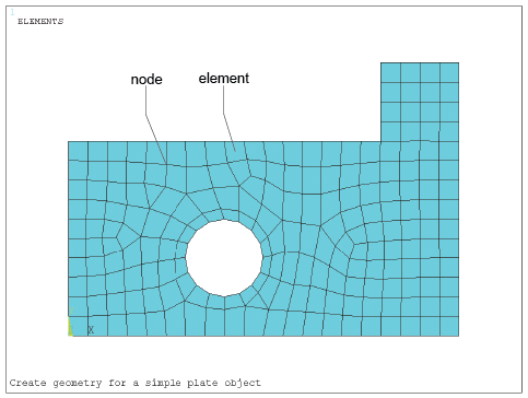
The complete set, or assemblage of elements, is known as a mesh . The process of representing a component as an assemblage of finite elements, known as discretisation, is the first of many key steps in understanding the FEM of analysis. An example is illustrated in Figure 1. This is a plate-type component modelled with a number of mostly rectangular(ish) elements with a uniform thickness (into the page or screen) that could be, say, 2 mm.
The field variable, e.g. temperature, is probably described throughout the body by a set of partial differential equations that are impossible to solve mathematically. Instead, we assume that the variable acts through or over each element in a predefined manner – another key step in understanding the method. This assumed variation may be, for example, a constant, a linear, a quadratic or a higher order function distribution. This may seem to be a bit of a liberty, but it can be surprisingly close to reality.
1.6 Outline of the finite element analysis process: structural analysis
The number and type of elements chosen must be such that the variable distribution through the whole body is adequately approximated by the combined elemental representations. For example, if the mesh is too coarse, the resolution of the parametric distribution may be inadequate, whereas too fine a mesh is wasteful of computing time and possibly the user’s time, and in some cases, won’t even solve anyway. Part of the skill will be in designing and refining meshes in areas of high interest or concentration of results variation gradients.
After model discretisation, i.e. subdividing the model domain into discrete elements (the mesh), the governing equations for each element are calculated and then assembled to give system equations. Once the general format of the equations of an element type (e.g. a linear distribution element) is derived, the calculation of the equations for each occurrence of that element in the body is straightforward. Nodal coordinates, material properties and loading conditions of the element are simply substituted into the general format. The individual element equations are assembled into the system equations, which describe the behaviour of the body as a whole. For a static analysis, these generally take the form , where, in structural problems, [ k ] is a square matrix, known as the global stiffness matrix, is the vector of unknown nodal displacements (or temperatures in thermal analysis) and is the vector of applied nodal forces (or heat flux in thermal analysis). The equation is directly comparable to the equilibrium or load–displacement relationship for a simple one-dimensional spring we invoked previously, where a force F produces or results from a deflection u in a spring of stiffness k . To find the displacement caused by a given force, the relationship is ‘inverted’, i.e. u = k −1 f .
The same approach applies to the FEM using . However, before the equation can be ‘inverted’ and solved for , some form of boundary condition must be applied, as we’ve seen. In stress problems, the body must be restrained from rigid body motion. For thermal problems, the temperature must be defined at one or more nodes. The solution to the equation is not trivial in practice because the number of equations involved tends to be very large. It is not unreasonable to have 250 000 equations, and consequently [ k ] cannot be simply inverted – there is unlikely to be enough computer memory to store all the numbers and data.
Fortunately, as we’ve seen, [ k ] will probably be banded, i.e. terms are grouped about the leading diagonal of the matrix, and more ‘distant’ terms will be zero. Techniques have been developed to take advantage of these features to store and solve the equations efficiently without going through an ‘inversion’ process. Remember that we are generally solving for the nodal displacement values first; it is then a simple matter (using a computer package) to use the displacements to find the strains and then the elemental stresses, via the appropriate Hooke’s law and strain/stress (constitutive) relations.
The major stages in the creation of any finite element model, according to Baguley and Hose (1997), for most types of analysis are:
- selection of analysis type
- idealisation of material properties
- creation of model geometry
- application of supports or constraints
- application of loads
- solution optimisation.
It is extremely important to:
- develop a feel for the behaviour of the structure
- assess the sensitivity of the results to approximations of the various types of data
- develop an overall strategy for the creation of the model
- compare the expected behaviour of the idealised structure with the expected behaviour of the real structure.
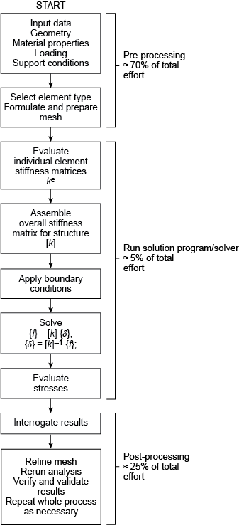
For those of us who like pictorial representations, think of the process as shown in Figure 2. Note the estimated proportions of time and effort that are (or should be!) spent in the various phases of preprocessing, solution and post-processing.
1.7 Hints and tips on finite element analysis
Don’t rely on one run. Refine the mesh in areas of high stress, repeat two or three times, check the iteration effects.
Remember that we are only ever solving a model of the real problem.
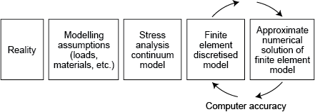
A good finite element model, once set up, is about a 95% accurate solution of the field equations, which themselves are based on a theoretical model, which is idealised from reality, and which uses assumed material properties (Figure 3).
Don’t confuse the processing accuracy of the computer with the validity of the solution.
Computer-aided FEA makes a good engineer better – it makes a bad engineer dangerous !
Finite element model solution (outline)
Here is a reminder of the main steps involved in the FEA of a structural problem.
Pre-processing stage
The component under investigation is ‘discretised’ into an assembly of finite elements in the prerocessing stage, with particular reference to the following six aspects.
- Element boundaries should coincide with structural discontinuities.
- Points of application of forces (and restraints) must coincide with suitable nodes, and any abrupt changes in distributed loading must occur at element boundaries. (Pressures are applied to the centroids of element faces.)
- Nodes should be at the points of interest for which output data are required, e.g. displacements, reaction forces, etc.
- The selection of element order (e.g. linear, parabolic, cubic) defines the interpolation or shape function of displacements between nodal points, i.e. the order of a polynomial in x , y and z directions, and hence the variation of stress/strain. Furthermore, the element type (e.g. spring, rod, beam, triangular and quadrilateral planar or shell, tetrahedral or hexahedral (brick) element) needs to be chosen. Often, the expected behaviour and physical shape of the component being analysed will guide the selection.
- Boundary conditions (e.g. applied loads, fixed nodes and restraints) and material properties must be entered. Loads and restraints are often the most difficult parameters to represent accurately, and have a significant influence on the predictions.
- Extensive model checks for cohesiveness, clashes, ‘cracks’, aspect ratios of elements, etc., must be carried out.
Solution stage
The fundamental unknowns to be solved are displacements u , v and, for fully three-dimensional analysis, w , for each node, with reference to a global frame of reference. Other data such as stresses and restraint reaction forces are calculated from these solution displacements, via the strains, at a later stage in the computation.
Within each element, a set of virtual displacements is applied and expressed in terms of the unknown displacements of the nodes. An element stiffness matrix is formulated using a numerical integration technique on the basis that actual displacements occurring will be those that minimise the strain energy. (This minimising of a functional parameter as a convergence criteria is an example of the calculus of variations.)
The individual element stiffness matrices are then combined to form a global stiffness matrix for the whole body from which a vast field of linear algebraic equations relating nodal forces, element stiffnesses and nodal displacements are formed. Boundary conditions are applied to the relevant nodes and the displacements and are then solved using numerical techniques such as Gaussian elimination, Gauss–Seidel iteration or Cholesky square root methods. For each node connecting two or more elements, compatibility of displacements and equilibrium of forces are maintained at that node (although derivatives of the displacement interpolations generally are not continuous across interelement boundaries). The assembly of the global stiffness matrix and the solution of the displacement equations occupies most of the processing time.
Once a solution for the nodal displacements has been obtained (or in the case of iterative techniques, once satisfactory convergence is achieved for them all) for each element, the stresses are computed based on the material data entered, the original element dimensions and newly computed nodal displacements.
Post-processing stage
The results of the solution are given in the form of stress plots (e.g. maximum principal, minimum principal, maximum shear, von Mises), deformed geometry (i.e. the distorted shape) and listings of nodal displacements ( u x , u y , u z ). Picture files can be created to obtain hard copies, or individual programs written to read the results file and carry out further data processing, if required.
1.8 A further few words of caution!
A successful FEA project requires properly executing at least three complex processes according to NAFEMS (2001):
- The user must be capable and qualified to pose a ‘question’ correctly to the software.
- The software must be mathematically robust and accurate enough to provide a good solution.
- The user must again be qualified to understand the results and assess the performance of the system based on these results.
While software vendors have gone to great lengths to make their codes accurate and easy to use, most users aren’t holding up their end by learning the techniques, engineering and discipline required to successfully use these products.
2 Case study
Formula 1 motor racing is a multi-billion dollar, high technology and highly competitive professional sport. In many ways it’s at the leading edge of car design - be it aerodynamics, electronics, materials or engineering. The best drivers compete on a world stage where fractions of a second mean the difference between winning and losing.
Enormous effort goes into the design, manufacture and testing of a racing car and all its components and systems – to gain those fractions of a second. The very latest tools and equipment are used to create the engineering components – usually with a rapid turnaround time and short production cycle. A modern Formula 1 car then is an ideal example to show engineering at its best.
The case study looks at the chassis tub, which not only houses and protects the driver but is the structure to which all the major components are attached.
The clips feature extensive contributions from Lewis Butler, Red Bull’s senior structural analyst, at the time of recording, and Dr Keith Martin of The Open University.
Transcript: Video 1
2.1 Modelling the tub of a Formula 1 racing car
The tub case study uses the same 7 steps approach as the hub case study but some of the steps and aspects are handled differently.
Transcript: Video 2
Let’s look at more detail on the construction materials of the tub.
Transcript: Video 3
Here are some more issues affecting the design of the tub.
Transcript: Video 4
Step 1 – The component
As with the hub, we’ll be looking at a specific load case for the tub - one which enables the team to compare new designs or modifications from one model to the next.
Before we can consider building a model of the tub we need to understand what it is – what does it do and how does it interact with other components on the car?
We’ll begin with Lewis describing the component.
Transcript: Video 5
The tub is made from carbon fibre composites. As a cocoon for the driver, it needs to be immensely strong and is subject to a range of impact tests to ensure that it meets the standards stipulated by the governing bodies of Formula 1.
We also know that all the car’s major components such as the engine are mounted directly onto the tub. And that the suspension members carry the forces generated by the wheels into the tub and out into the rest of the car.
Step 2 – The loads
Now the next thing to consider is what load case should we apply to our FEA model.
Transcript: Video 6
There are good reasons for being interested in the torsion test. The torsional stiffness of a racing car chassis is vital in determining overall performance, whatever it is made of.
Transcript: Video 7
Step 3 – Boundary conditions
The boundary conditions for the tub are quite straightforward. You may recall that the entire back end of the car - comprising the engine, gear box and so on – is attached solidly to the rear bulkhead of the tub. Other bits and pieces such as electrical wiring, controls, and water pipes we can forget about.
Transcript: Video 8
Step 4 – Modelling issues and assumptions
For both the boundary condition restraints and load input points we can expect some localised high stresses. We’re not interested in these though. As long as the loads and reaction forces are fed into the structure, the main part - the bit we’re interested in - will be modelled and behave close to the real thing.
For this component Steps 1, 2 and 3 are relatively easy, even easier than for the wheel hub.
Considering modelling issues and assumptions, the tub is large, of a complex shape, and made of a material which is clearly not isotropic. It is ‘orthotropic’.
Transcript: Video 9
If you compare the chassis tub to the hub, material behaviour is probably the most different aspect. The hub is made of steel, a linear, elastic, homogenous and isotropic material, and can be described using only a couple of numbers.
Transcript: Video 10
Step 5 – Building and solving the FEA model
In this step we must build the model. As it is so large and has complex material properties, we will only build half the model and use symmetry to solve it. A full model may take a very long time to solve, or may not even solve at all.
Transcript: Video 11
Transcript: Video 12
Step 6 – Post-processing the FEA model
Once it is solved, we go to the post-processing step to view the results of the calculations.
Transcript: Video 13
In this case, Lewis was only interested in the relative stiffness of the chassis tub, particularly any effects due to modifications in the driver area which was the weakest in terms of torsion.
Step 7 – Post testing and verification
The model can be adapted for each new car and any tests go towards verifying the computer model on a continuing basis.
Transcript: Video 14
The beauty of Red Bull’s approach to this model is that it is quite easy to match up with a real test and compare results.
The model itself has been refined over a few seasons and developed, based on subsequent testing of real tubs. This means the model can be used with confidence. Any improvements in torsional stiffness that it predicts are likely to be real.
Transcript: Video 15
The National Agency for Finite Element Methods and Standards (NAFEMS) says that it is a common mistake in computer analysis to assume that the output, or results, of a processing job are as valid as the processing accuracy of the computer.
Instead NAFEMS recommends that it is safest to consider a set of results to be wrong until you are sure that they are at least of the expected orders of magnitude. For example computed reaction forces agree closely with hand calculated values and so on.
Remember, the computer won’t tell you that you’ve modelled the restraints properly, or that the material properties are correct.
Transcript: Video 16
3 FEA exercises
Now is a good time to try out the FEA if you have access to FEA software. These exercises are designed to familiarise you with basic software capabilities.
3.1 Exercise: Analysis of a plate with a hole
Problem description
This is a simple problem with a known solution. It consists of a tensile-loaded thin plate with a central hole. Because of symmetry we need only model a quarter of the plate. The full plate is 1.0 m × 0.4 m with a thickness of 0.01 m. The central hole has a diameter of 0.2 m.
The plate is made of steel with a Young’s modulus of 2.07×10 11 N/m 2 and a Poisson’s ratio of 0.29. The horizontal tensile loading is in the form of pressure of 1.0 Pa (N/m 2 ), along the vertical edge of the full plate.
Interactive time required
60 to 70 minutes
Features demonstrated
Solid modelling, including primitives, Boolean operations, meshing and refinement.
Summary of steps
- Specify title
- Define parameters to be used for geometry input
- Set preferences
- Define element types
- Element options
- Define material properties
- Create rectangular area
- Create circular area
- Subtract hole from plate
- Mesh the area with a default mesh
- Apply displacement constrains
- Apply pressure load
- Solve
- Plot the deformed shape
- Plot the element stress in the x-direction
- Refine mesh
- Refine mesh near hole
- Re-introduce the loads
- Read in the new data set and plot the element stress in the x-direction
- Exit the program.
Interactive step-by-step solution
- Specify title
- Specify a title for your project.
- Define parameters to be used for geometry input
- HEIGHT = 0.20
- WIDTH = 0.50
- RADIUS = 0.10
- THICK=0.01
- Set preferences
- Make sure that Structural Analysis option is enabled.
- Define element types
- Choose an 8-node 1PLANE element (PLANE183).
- Define options for your element types
- Set the element options so that it behaves as ‘plane stress with thickness’.
- The thickness of the element should be set to 0.01.
- Define material properties
Set material properties to:
- Young’s modulus: 2.07 × 10 11
- Poisson’s ratio: 0.29
- Create rectangular area
- Create a rectangular area with
Width = WIDTH
Height = HEIGHT
- Create a rectangular area with
- Create circular area
- Create a circular area with centre at (0, 0) and Radius = RADIUS
- Subtract hole from plate
- Use Bollean operations to subtract the hole from the rectangle.
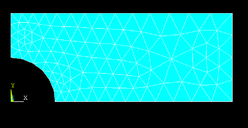
- Mesh the area with a default mesh
- Choose ‘Triangular elements’ for Shape.
- Click Mesh.
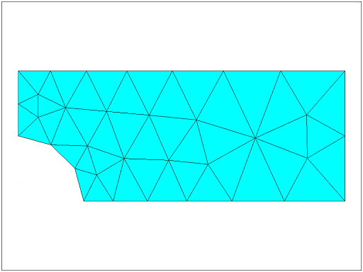
In this example we choose to mesh with triangular elements.
It should look something like this:
- Apply displacement constraints
The boundary conditions we apply must represent the symmetric nature of the problem.
Note: we are going to do this in two distinct steps as an illustration of applying a simple fixed displacement to the nodes attached to a line. In this case, however, as the displacements are equal, i.e. zero, we could have done this in a single step.
- Apply structural displacement BC to the left edge of the model.
- Pick UX (x- direction displacement).
- Enter 0 for Displacement Value.
- Apply structural displacement BC to the bottom edge of the model.
- Pick UY (y-direction of the displacement).
- Enter 0 for Displacement Value.
Alternative route:
You can achieve the same result by applying a symmetry boundary condition on left-most and bottom edges.
- Apply pressure load
The unit pressure load will be applied to the line at the right.
- Apply a structural pressure load right-hand edge (line 2).
- Enter –1.0 for ‘Load Pressure’ value (this ensures that the pressure is outwards as we have a tensile load).
- Solve
- Solve the arrangement.
- Plot the deformed shape
- The maximum displacement is given as DMX = 0.321 × 10⁻¹¹. This seems reasonable for a unit load.
- Plot the element stress in the x direction
The element stress is a good thing to look at after the displacement. It will show us any steep gradients.
Note that we have rather steep gradients in the area of concern around the hole.
We will address this by refining the mesh.
- Refine mesh
This command will subdivide all the elements.
However, in some programs before refining the mesh we need to remove the loads.
The resultant global refinement is given below. Compare this mesh with the one above.
- Refine mesh near hole
You should refine further around the top of the hole.
- Select the three nodes at the top tip of the circular cut.
- Refine the mesh in these elements/nodes.
This produces more elements in the area of interest.
- Re-introduce loads and Solve
Repeat steps 11 and 12 above to add load, then solve.
- Read in the new data set and plot the element stress in the x-direction
- Choose X-Component of stress to plot.
The stress contours are now smoother across the element boundaries and the stress legend shows a maximum value of 4.39 Pa. We must check these results. Find the theoretical stress concentration factor, K t , for this problem in any good source. We determine that for this geometry, K t = 2.17. The maximum stress is given by:
( K t )(load)/(net cross sectional area)
Using a pressure of p = 1.0 Pa we get:
σ x, MAX = 2.17× p ×(0.4)(0.01)/[(0.4-0.2)*0.01] = 4.34
The computed maximum value is 4.38 Pa which is less than 1% in error, assuming that the value of K t is exact.
- Exit the program.
3.2 Exercise: Cantilever beam
Problem description
The problem is a simple cantilever beam. We only give outline instructions for most of this problem. You are required to issue the correct commands, based on your previous experience and the given data.
At the end of this exercise you are asked to use your knowledge in beam theory to calculate the bending stresses and to verify the results of your finite element analysis.
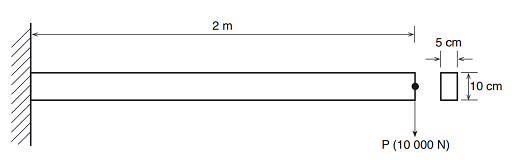
Figure 6 illustrates the problem and associated dimensions. Note that all dimensions should be converted to millimetres and appropriate units for the analysis. Recall that it is the user’s responsibility to insure that all units are consistent! The boundary conditions consist of fully fixing the node on the left.
The applied load is a single point load (force of 10000 N) applied to the right node of the beam. The relevant dimensions are as follows:
Length = 2 m
Depth = 10 cm
Width = 5 cm
The beam is made of steel with a Young’s modulus of 200 GPa and Poisson’s ratio of 0.30.
Origin
University of Alberta, MECE.
Interactive time required
45 to 60 minutes.
Features demonstrated
Linear analysis, Solid modelling, Meshing, Element table data, Post processing.
Summary of steps
- Set title and preferences
- Define element types and options
- Define material properties
- Define beam section parameters
- Create 2 Keypoints
- Create a line
- Set Global element edge size
- Mesh the line with a default mesh
- Apply displacement constraints
- Apply Force load
- Rotate axes
- Solve with default criteria
- Plot deformed shape
- List nodal displacement values
- List stresses in the beam
- Validate your results
- Exit the program.
Interactive step-by-step solution
- Set title and preferences
Give your job a title, e.g. ‘Cantilever Beam’.
- Define element types and options
Select a 2d elastic beam element.
Is this a good element choice? You can also look at the options for this element type.
- Define material properties
Set Young’s modulus to 2.× 10 5 (in units of N/mm 2 ) and Poisson’s ratio to 0.3
- Define beam section parameters
- set 50 for width and 100 for height.
Note that the vertical axis here is the z -axis, so the force will be applied in the z direction.
It is also a good idea to preview the section data summary to check that all the parameters are entered and calculated correctly.
The parameters of interest are:
Area = B × H = 5000
Second moment of area about y -axis
= I yy = B ×( H 3 )/12 = 0.41667× 10 7
- Create 2 Keypoints
Create two key points at:
KP 1 = 0, 0, 0
KP 2 = 2000, 0, 0
- Create line
Create a line between these two key points.
- Set global element edge size
Set global element size to 200
- Mesh the line with a default mesh
Mesh the line.
- Apply displacement constraints
Fix all dofs at key point (or node) number 1
- Apply force load
Apply a force of 10000 N in the minus Z direction on the node at the other end of the beam.
- Rotate the axes
If necessary, rotate the axes so that the z-axis is pointing up:
- Solve with default criteria
Solve the system.
- Plot deformed shape
What is the maximum displacement at the tip?
I got 32.0 mm
- List nodal displacement values
Here is the list of displacements I obtained as a function of node x-position:
| Node number | Node x-position | Displacement (Uz) |
| 1 | 0 | 0.000 |
| 3 | 200 | 0.4637 |
| 4 | 400 | 1.7914 |
| 5 | 600 | 3.8872 |
| 6 | 800 | 6.6549 |
| 7 | 1000 | 9.9986 |
| 8 | 1200 | 13.822 |
| 9 | 1400 | 18.030 |
| 10 | 1600 | 22.526 |
| 11 | 1800 | 27.213 |
| 2 | 2000 | 31.997 |
You can see that the maximum displacement is 32 mm (to 2 dp).
- List stresses in the beam
To look at the stresses in the beam we normally need to define an element table. You should read your FEA software’s help menu, particularly on your chosen element to determine the name (or identifier) of variables that give bending stresses.
I obtained the following values of axial and bending stresses for each element:
| Element number (from constrained end) | Axial stress | Bending stress (stresses in both nodes are computed to be the same) |
| 1 | 0.00 | -228.0 |
| 2 | 0.00 | -204.0 |
| 3 | 0.00 | -180.0 |
| 4 | 0.00 | -156.0 |
| 5 | 0.00 | -132.0 |
| 6 | 0.00 | -108.0 |
| 7 | 0.00 | -84.00 |
| 8 | 0.00 | -60.00 |
| 9 | 0.00 | -36.00 |
| 10 | 0.00 | -12.00 |
- Validate the bending stresses
Now you need to use your knowledge in beam theory to verify the results of your FE model. Follow the procedure below:
- Draw a free body diagram of your beam and calculate the bending moment at the ends of each element.
- Calculate the second moment of area about y-axis, I yy = B ×( H 3 )/12
Calculate the maximum bending stress at the ends of each element using the classic Engineer’s Bending Equation,
For example, for element 1 you should get bending stresses of 240 MPa at node I and 216 MPa at node J which gives the average stress of 228 MPa for element 1. This is exactly what we achieved from your finite element model.
- Exit the program.
Conclusion
In this course you were introduced to the FEA process or method. We outlined the many continuum fields and subjects in which FEA can be applied and showed how modelling using FEA is now an important part of engineering.
This course demonstrated the importance of understanding the limitations and assumptions involved in order to use FEA safely with the aid of some tips and words of caution.
Formula 1 motor racing is at the leading edge of car design – be it aerodynamics, electronics, materials or engineering. The important role that FEA plays in Formula 1 car design is highlighted in a case study involving the tub (body) of a racing car.
Finally, to drive home the importance of practice of FEA, two simple exercises are explained in detail so that, provided you have access to FEA software, you can begin to understand the capabilities of the software.
Today, engineers use computers and software in the design and manufacture of most products, processes and systems. Finite element analysis (FEA) is one of the most important tools in an engineer or designer’s arsenal of digital tools for design and analysis of products and processes. This course has given you a brief introduction to the finite element method and the need for comprehensive evaluation and checking when interpreting results.
References
Acknowledgements
Except for third party materials and otherwise stated (see terms and conditions ), this content is made available under a Creative Commons Attribution-NonCommercial-ShareAlike 4.0 Licence .
Course image: Jonathan Lin in Flickr made available under Creative Commons Attribution-ShareAlike 2.0 Licence .
The material acknowledged below is Proprietary and used under licence (not subject to Creative Commons Licence). Grateful acknowledgement is made to the following sources for permission to reproduce material in this free course:
Every effort has been made to contact copyright owners. If any have been inadvertently overlooked, the publishers will be pleased to make the necessary arrangements at the first opportunity.
Don't miss out
If reading this text has inspired you to learn more, you may be interested in joining the millions of people who discover our free learning resources and qualifications by visiting The Open University – www.open.edu/ openlearn/ free-courses .