

4.3.5 Choosing statistical tests (OPTIONAL)
This section is optional in that it provides more detail on the statistical tests that can be applied to analyse the data. If you have time and/or such analysis is important to the type of work you do, you should study this section.
Many different statistical tests have been developed, and we will only look at the most common ones in this module. Firstly, statistical tests can be classified as
We will look at two categories of tests in this section. First, let us consider the tests to use when the exposure variable is a categorical variable. In this case, statistical tests allow us to assess differences between counts or means of the outcome variable at different levels of the exposure variable (e.g. assess the differences in average healing time (outcome variable) for different treatments A, B and C). The choice of such a statistical test depends on the type and characteristics of the data being analysed. One way to determine what test is most appropriate is to identify the type of outcome variable, the number of groups being compared (i.e. in our example – there are three levels of the variable ‘treatment’: A, B and C) and whether the assumptions for the test are met (this step may be informed by the descriptive analysis). Table 6 lists the most important assumptions for each test. For example, a non-parametric Mann-Whitney test might be used to test whether there are differences in the presence of AMR genes in bacterial isolates sampled from patients in hospitals, compared to patients in the community.
Statistical tests in a second category are those used when the exposure variable is numeric. In this case, tests allow users to assess the existence of a significant relationship between the (numeric) outcome and exposure variables. When there are no other variables to consider, such a test is called a correlation or collinearity test. The most commonly used correlation tests are Pearson’s r (parametric, normally distributed variables) and Spearman’s ρ rank correlation (non-parametric). For example, researchers conducting a multi-country study have data on the prevalence of resistance to a particular antimicrobial for two target organisms for 20 countries. If they want to know whether resistance to a particular antimicrobial in one target organism is related (correlated) to resistance in the second target organism, they could use a test for correlation. If additional variables need to be considered in the analysis, multivariable regression models can be constructed, though this is beyond the scope of this module.
Table 6 provides an overview of the types of statistical tests you can conduct according to the type of data you have. If you’re just starting out in learning statistics, some of this information might seem very complex, but you don’t need to understand it all now. Keep a copy of this table for future reference for when you plan and conduct your own analyses of AMR data. An important point to note for now is that results obtained from statistical tests are only valid when all the assumptions for the test are met. This important point is not always easy to assess in practice. Two important assumptions common to the seven tests presented in Table 6 are that the observations are based on a random sample and that they are independent from each other. When observations are not independent, for example, when several observations are obtained from the same individual at different points in time (repeated observations) or from a matched study design, then other tests should be used, such as paired sample t-test or mixed-effect regression models. Such tests are out of the scope of this course.
| Parametric or non-parametric? | Outcome variable | Number of groups Footnotes 1 | Statistical test | Key assumptions |
|---|---|---|---|---|
| Parametric | Categorical: nominal with two levels (dichotomous) | Two or more | Chi-squared test | Expected frequency in any cell of a contingency table is not |
| Non-parametric | Categorical: ordinal, or numeric when assumptions for a t-test are not met | Two groups | Mann-Whitney U test (Wilcoxon rank-sum test) |
|
| Non-parametric | Categorical: ordinal, or numeric when ANOVA test assumptions are not met | Three or more groups | Kruskal-Wallis test | Outcome can be ranked |
| Parametric | Numeric | Two groups | Student’s t-test |
|
| Parametric | Numeric | Two or more groups | One-way ANOVA |
|
| Parametric | Numeric | Two or more groups | Simple linear regression with one exposure variable |
|
| Parametric | Categorical: nominal with two levels (dichotomous) | Two groups | Binomial logistic regression | Linear relationship between the exposure and log odds |
Footnotes
Footnotes 1This is the number of groups being compared i.e. the number of levels in the exposure variable. Back to main text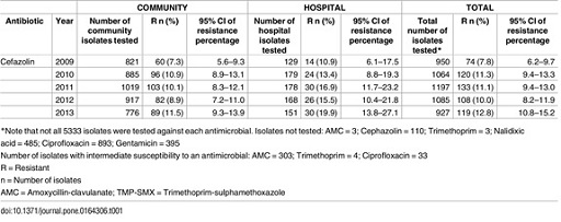
Activity 8: Conducting a statistical test
- Draw a simplified two-by-two contingency table with only the count values that are of interest for the first part of this activity (comparing 2009 with 2010) from the data presented in Figure 5.
Hint: the contingency table should show the number of isolates with were identified as resistant and the number identified as susceptible in each year, in all settings.
Answer
| Isolate status | Year 2009 | Year 2010 |
|---|---|---|
| Resistant | 74 | 120 |
| Susceptible | 876 | 944 |
The number of susceptible isolates each year was obtained by removing the number of resistant isolates from the total number tested, i.e. 950 and 1064 isolates in 2009 and 2010, respectively.
- Using an online calculator for carrying out Chi-squared tests (such as this one), use the data above to perform a Chi-squared test.
Hint: if you made your table in Excel, just copy and paste into the calculator. Alternatively, you can enter the data by copying and pasting the text below:
| Isolate status | Year_2009 | Year_2010 |
|---|---|---|
| Resistant | 74 | 120 |
| Susceptible | 876 | 944 |
Answer
The p-value obtained from the test is 0.010, indicating that there is a statistically significant difference between the proportion of resistant isolates in 2009 and in 2010. Note that the result also presents the Chi-squared statistic (which is 6.62) and degree of freedom (which is one) – these parameters are used to calculate the p-value, but apart from recognising that Chi-squared tests are suitable for data where the outcome variable is categorical (Table 6), you don’t need to understand more about these parameters in this module.
- Do the same test to compare the proportion of resistant isolates between 2010 and 2011.
Answer
The Chi-squared statistic for this second comparison is 0.003, with one degree of freedom. The p-value obtained from the test is 0.95, indicating that there is no evidence for a statistically significant difference between the proportion of resistant isolates in 2010 and in 2011.
4.3.4 Limitations of null hypothesis testing
