2.1.2 Variables

A variable is any characteristic or attribute of a data unit that can be measured. The term variable is used because the value can vary from one data unit to another and may change over time. Examples of commonly used variables used to characterise a patient in a hospital include ‘age’, ‘gender’, ‘date of admission’, ‘body temperature at admission’, ‘primary diagnosis’, etc. Variables that might be used to characterise an individual animal might include ‘age’, ‘sex’, ‘breed’, ‘production type’, ‘farm identification number’, ‘herd size’ and others. Variables relevant to a laboratory that performs AST might include ‘date of sample’, ‘specimen identification number’, ‘sample type’, ‘minimum inhibitory concentration’ and many others.

Some variables can be observed or recorded directly – for example, the body temperature of a person or animal can be observed by reading the result on the thermometer, providing it is working and used correctly. Other variables are defined by applying rules or calculations to directly observed variables. For example, the variable ‘fever’ might be based on a binary classification of body temperature, with any patients recording a body temperature higher than 37.5°C classified as having a fever, while those with a body temperature of 37.5°C or less classified as ‘no fever’. Similarly, ‘age in years’ can be recorded directly or calculated from the documented date of birth.

Variables can be further classified into numeric (quantitative) and categorical (qualitative) variables. This has implications for how much information is conveyed by data, and how it can be analysed.

Consider once more the example of body temperature. Imagine that you measure the body temperature of five patients using a standard thermometer, with the results shown in Table 2.

Now imagine that you have data for the same patients, but this time the data is represented using the variable ‘Fever’, which has two categories, ‘Yes’ and ‘No’. Their body temperatures are shown again in Table 3. A cut-off value of 37.5°C or above is used to determine whether the patient has a fever.

By now you can probably infer some of the key differences between numeric and categorical variables. Numeric (quantitative) variables have the following characteristics:

• data are represented as counts or measurements
• data are represented using numeric values as integers (1, 2, 3), fractions (½, ¼) decimals (37.7, 39.134) or percentages (20%, 50%)
• include age, height, blood pressure and minimum inhibitory concentration.

Categorical (qualitative) variables have the following characteristics:

• data are represented as belonging to a particular group (a ‘category’)
• can be represented by a name, a string of alphanumeric characters, or numeric values
• include sex/gender, occupation and antimicrobial class.

In addition to classification as ‘numeric’ or ‘categorical’, variables are further defined by what they measure (see Figure 1).

Figure 1 Variable classifications.

Show description|Hide description

A tree diagram that summarises different types of variable. ‘Variable’ at the top is divided into numeric (quantitative) and categorical (qualitative) variables, and then ‘Numeric’ is divided into continuous and discrete variables, and ‘Categorical’ into ordinal and nominal ones.

Figure 1 Variable classifications.

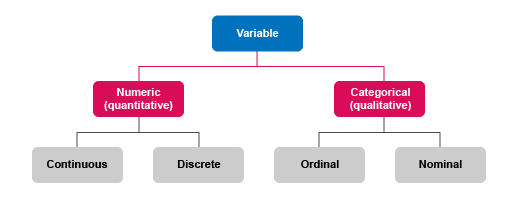
Numeric variables can be either continuous or discrete.

Continuous variables:

• represent measurements that can take any value within a range
• can be recorded using integers, fractions, percentages or decimals
• examples include milligrams of antimicrobial ingredient per kilo of bodyweight.

Discrete variables:

• represent counts of individual items or values
• are always recorded using integers (whole numbers)
• examples include the number of animals in a herd, number of different antimicrobials to which resistance is identified.

Categorical variables can be either nominal or ordinal.

Nominal variables:

• are classified into two or more categories that are mutually exclusive
• have no intrinsic order or ranking, or distance between the values
• when there are only two categories, this is known as a ‘dichotomous’ or ‘binary’ variable
• examples include antimicrobial class, pregnancy status and all yes/no questions.

Ordinal variables:

• comprise three or more categories that are ‘ordered’ or ‘ranked’, so that one value is ‘larger’ or ‘smaller’ than another value
• the distance, or gap, between values is not necessarily equal
• examples include body mass index (BMI) category (underweight, normal weight, overweight, obese) and resistance category (susceptible, intermediate, resistant).

The reason that variable classifications matter is that each one affects how data can be analysed, interpreted and used. You’ll learn more about this in the Processing and analysing data module. The key takeaway for this module, however, is to recognise that variable classifications are partly determined by the nature of the data unit that is being measured (for example, you can’t have half a person, so counts of people or animals are always discrete), and partly determined by how data are processed (such as when categorical variables are generated from continuous variables).