Appendix 2: Teacher notes - outputs of the lesson (Exploring the properties of electrons using a fine beam tube)
Appendix 2: Teacher notes - outputs of the lesson
The fine beam tube is a challenging experiment that draws on a number of different concepts delivered in SHS Physics Year 2. It would be worth using it only after teaching all of the material listed below. Alternatively, it could be delivered in Year 3 as a vehicle for revising these concepts.
|
Section |
Unit |
Objectives |
Content |
|
2 Mechanics |
1 Energy |
2.1.1, 2.1.2 |
Energy and conservation of energy |
|
|
2 Circular motion |
2.2.2 |
Centripetal force |
|
5 Electricity and magnetism |
2 Magnets |
5.2.2 |
Magnetic field |
|
|
3 Electro-magnetism |
5.3.1 |
Magnetic fields created by current |
|
|
|
5.3.2 |
Fleming’s Left- Hand Rule |
|
|
|
5.3.6 |
Force on a charged particle in a magnetic field and Electric field |
|
6 Atomic and nuclear physics |
2 Thermionic Emission |
6.2.1, 2 |
Thermionic emission and cathode rays |
Comments on Background
The fine beam tube (FBT) is an application that uses thermionic emission to produce an electron beam (Unit 2 Objectives 6.2.1, 2). The electric field forces in the anode accelerate the electrons and their speed can be calculated by conservation of energy (Unit 1, 2.1.1,2) such that the electrical work done accelerating the electrons = gain in kinetic energy.
The two coils produce a magnetic field between them (Unit 3, 5.2.2, 5.3.1). The field produces a force on the electrons, the direction is given by Fleming’s Left Hand Rule (Unit 3, 5.3.2) and the magnitude of the force using the formula given in Unit 3, section 5.3.6. Since the direction of the force is perpendicular to the velocity of the electrons, the force provides a centripetal acceleration (Unit 2, section 2.2.2) making the electrons travel in a circle.
However, the Helmholtz configuration is not introduced in SHS Physics, so this is an extension exercise, which serves as a synoptic task. By combining the equations given in these sections with additional equations for the specific magnetic field here, it is possible to derive a framework to investigate the relationship between
- The voltage used to accelerate the electrons (linked to their speed), V
- The current in the coils (which causes the magnetic force), I
- The radius of the electron beam, r
The exemplar shows how one relationship can be investigated graphically. At a higher level, the data can be used to determine the charge to mass ratio of an electron , using a single set of data or the gradient of a graph
Comments on Practical Activity
This section starts with a detailed account of the apparatus and its parts. The experiment is an Interactive Screen Experiment which is based on many photographs of a real set of apparatus showing all possible combinations of current, voltage, polarity and the resulting beam. Changing a slider changes the image smoothly to a different image with a different set of parameters so is close to running the experiment for real.
Comments on Investigating the Beam
This is a series of three short tasks to qualitatively investigate the behaviour of the beam, changing the voltage, current and polarity. For some student groups, it may only be sufficient to explore this task.
Comments on Making Measurements with a circular beam in the FBT
This is the quantitative investigation. It explains the data collection, graph plotting and calculation of
Using just data and graphically. These tasks build in difficulty so that the teacher can decide which tasks are appropriate to their students.
The algebra may be on the limit of what students are prepared for and has been simplified as much as possible to calculate Students will need access to a scientific calculator (e.g., one on a computer) as they will manipulate small numbers written in scientific notation and plot small numbers on the graph.
Mathematical background
Symbols used:
V = accelerating voltage
q = charge on a particle
e = charge on an electron = 1.602 × 10⁻¹⁹ C
m = mass of a particle
me = electron mass = 9.109 × 10⁻³¹ kg
v = velocity of an electron
B = magnetic field
F = force
r = radius of circular beam
= angle between magnetic field and velocity, 90° in this context
ratio = e/me = 1.76 × 10¹¹ C kg-1
N = number of turns of wire in each of the coils = 130 here
R = radius of each coil = 15 cm here
μ0 = permeability of free space = 4 π × 10-7 T m A-1
k = coils constant = T m-1 for these coils
Work done on electron = gain in kinetic energy.
Work done accelerating through and mass
The magnetic field force where and
The magnetic field provides the centripetal force,
From (2)
Using (1)
In the language used here, where
(3)
The last step is the relationship between B and I. The theory here is well beyond the level of SHS, so here is the given formula.
This is simplified to where
For this coil, R = 15.0 cm = 0.0150 m and N = 130 terms. Hence the coils constant = T m-1 for this apparatus
The final formula that links the experiment
This can be used as the basis of any investigation where you might want to fix one of (V, I, r) and vary/measure the other two.
Sample dataset
The experiment has three variables – V, I and r. It is possible to choose a constant value of one and investigate the relationship of the other two. Here, the instructions investigate the relationship between V and r (V∝ r2) with a fixed current as it is the easiest process to explain. It is possible to do two more investigations fixing r or V. The data can be manipulated into a straight-line graph for either of these combinations and the gradient used to determine . This could also be a planning exercise for some students.
Current I = 1.52 A
|
Voltage / V |
Left position /cm |
Right position / cm |
Diameter / cm |
Radius / m |
Radius2 / m2 |
|
130 |
10.3 |
16.0 |
5.7 |
0.0285 |
0.00081 |
|
150 |
10.3 |
16.5 |
6.2 |
0.0310 |
0.00096 |
|
170 |
10.3 |
17.0 |
6.7 |
0.0335 |
0.00112 |
|
190 |
10.3 |
17.3 |
7.0 |
0.0350 |
0.00123 |
|
210 |
10.3 |
17.7 |
7.4 |
0.0370 |
0.00137 |
|
230 |
10.3 |
18.0 |
7.7 |
0.0385 |
0.00148 |
|
250 |
10.3 |
18.3 |
8.0 |
0.0400 |
0.00160 |
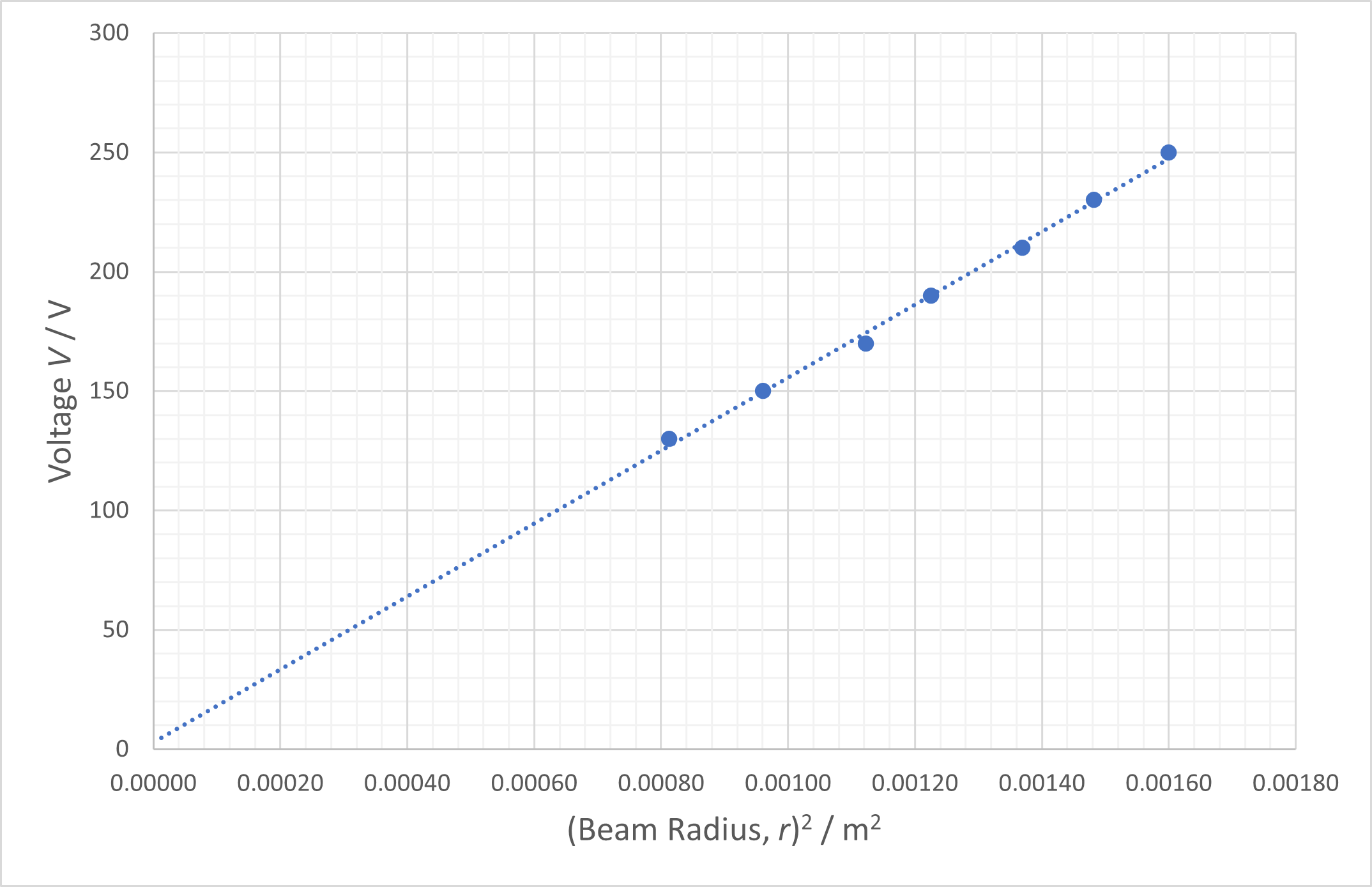
Graph showing Voltage against (Beam Radius)2 for the Fine Beam Tube, current fixed at 1.52 A
The gradient is 1.53 × 10⁵ V m-2
Sample single calculation of
Using the last row of the table and the answer to ITQ 6
Sample calculation from graph
Using the answer to ITQ 7, B calculated above and the gradient of the graph
Final value of and uncertainties
The calculated value of in this experiment is consistently higher than the established value of 1.76 × 10¹¹ C kg-1. With care, it is possible to get a graph showing a good straight line of best fit, through the origin, with little scatter around the line. There is plenty of scope for considering the uncertainties in the measurements of beam radius, voltage and current. There is scope to instruct students to repeat measurements of the radius.
The diameter of the coil and number of turns in each coil uses values provided by the manufacturer. They in turn are used in the calculation of used to determine the value of the magnetic field. That assumes that the separation of the 2 coils and alignment is as close as possible to the ideal Helmholtz configuration.
Extension questions
Below are some extension questions you may wish to use with your more advanced students.
Question A
Why does an increase in the coil current lead to a smaller radius for the electron beam?
Answer for Question A
The magnetic field is proportional to this current so it increases. The force provides a stronger centripetal force, which in turn is inversely proportional to the radius of the path. So, a stronger field supports a smaller circle for constant velocity.
Question B
Why would you not be able to perform this experiment with a vacuum in the vacuum tube?
Answer for Question B
You would not be able to see the electron beam. The faint lilac glow of the beam arises from collisions between the electrons and hydrogen atoms. The electron within the atom is excited to a higher energy level
Question C
Why did we ask you to do experiments with quite small circles, radius up to about 4 cm?
Answer for Question C
The Helhmoltz configuration of two coils is about as good as a physicist can do to produce a uniform magnetic field. It is extremely close to uniform for a cylindrical region between these coils up to a radius up to about 4 cm from the axial line through the centre of the 2 coils. Thereafter, it decreases significantly. This experiment is constrained by having the beam within the region which shows the most uniformity. So, we asked you to use a current of about 1.5 A to limit this
You could use a bigger current and smaller circles, but that may not give the best results. The beam can only be measured with limited precision (e.g. random uncertainty of ± 1 – 2 mm, so a smaller radius would have a larger percentage of fractional uncertainty).
More challenging questions
Question D
Calculate the velocity of the electron using your value of when the accelerating voltage = 220 V.
Hint – the electrical energy given to the electron is its charge × voltage and this is converted into kinetic energy
Answer for Question D
Using
Rearrange for
Example, with and
So, the voltage accelerates the electron to almost 10 million m s-1.
Question E
Calculate with the following data – = 220 V, =1.60 A, = 0.040 m
Answer for Question E
Using
First work out B
Rearranging (1) and using the value for B
Previous: Appendix 1 Next: Lesson: Investigating the properties of electrons using a fine beam tube