Background

Fieldwork

Fieldwork can be rewarding and enjoyable. Before starting, it is always useful to plan carefully what you intend to do in the field.

Fieldwork can be divided into three main stages:

• careful observation
• recording what you can see or measure
• analysis and interpretation.

When you go on a field trip you observe and record what is going on in the environment. Recording data and observations in an organised way is a key skill. It is better to record more observations than you think you will need, rather than risk recording too few. You can always ignore extra notes when working with your data back in the classroom, but often you cannot go back to make further observations. You should record the location and date of every field observation.

Qualitative observations are recorded in words, but also as images such as photographs and sketches. You can include subjective terms, such as descriptions of colour and shape; for example, the tree has fan-shaped leaves with spiny edges and hard, yellow fruit. Quantitative observations are records of numerical values obtained from measurements or by counting, for example, the silk cotton tree is 50m tall or there are 5 plant species in this 1 m² area.

You can develop observational skills through practice – if you get used to noticing different types of plants or animals, you will start to spot patterns in the environment that are not apparent to an untrained eye.

Making a field sketch

Careful field sketches always form a key part of field notes and are important in developing observational skills. Field sketches are not perfect drawings; your aim when drawing a field sketch is to highlight the important features. Sketches, unlike photographs, are interpretations, as the act of sketching makes you think about which features to include and which to leave out. You should annotate your field sketch with observations. You can include biotic features (such as plants and animals and descriptions of vegetation and habitats), abiotic features (such as water and rocks) and features that show human impacts (such as buildings, paths, machinery, agriculture and pollution).

Figure 1 below shows a view from the virtual field trip with an annotated field sketch of the same view.

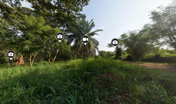
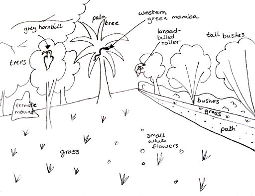
Figure 1. (a) A view of an environment showing different types of vegetation in the Palm tree site panorama in the Legon Botanical Gardens, Ghana. (b) An annotated field sketch of the same view with labels recording relevant information about observations in the environment.

Different organisms live in different places. The term habitat means the place where an organism lives. It describes an area in the landscape which supports a particular group of organisms, for example, a grassland habitat is one that is mainly made up of grasses, a woodland habitat is dominated by trees and a lake habitat supports aquatic organisms. These can also be subdivided into more specific habitats, for example, a mangrove forest is dominated by a particular tree species – the mangrove tree.

What are the main points to remember when making a field sketch?

To highlight the important features and to annotate your drawing with observations.

Hierarchy of living organisms

Individual organisms are named and sorted into a hierarchical system. This is intended to reflect evolutionary relationships, like a huge ‘family tree’ stretching back millions of years. The hierarchy of categories is shown in Figure 2.

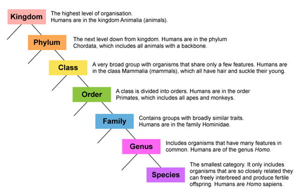
Figure 2. Hierarchy of living organisms

At the lowest level is the species – each species has a scientific binomial name, printed in italics. The first part of the name is the genus, which always starts with a capital letter. The second part is the species, which never starts with a capital letter. For example, humans are known scientifically as Homo sapiens.

Many, but not all, organisms also have common names. The difficulty is that these common names can vary in different regions or countries. The scientific binomial name is a unique name that is recognised across the world.

The following tables show the taxonomy of two organisms that are not closely related (Table 1) and two that are closely related (Table 2).

Table 1. Taxonomy of two organisms that are not closely related: an animal (kob) and a plant (silk cotton tree)

Taxa	Organism 1	Organism 2
Kingdom	Animalia	Plantae
Phylum	Chordata	Trachaeophyta
Class	Mammalia	Magnoliopsida
Order	Artiodactyla	Malvales
Family	Bovidae	Malvaceae
Genus	Kobus	Ceiba
Species	kob	pentandra
Notes:	Kobs are antelopes found in Central, West and East Africa. They have reddish-brown fur with a white eye-ring, inner ear and throat. They are diurnal (active during the day) but inactive during the hotter hours. Males have horns and females do not.	The silk cotton or kapok tree is a tall tree (up to 50m), with buttresses at the roots and large spines sticking out of the trunk. The kapok has woody pods containing a white, fluffy seed covering.

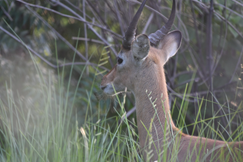
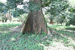
Table 2. Taxonomy of closely related organisms (ring-necked parakeet and African grey parrot)

Taxa	Organism 1	Organism 2
Kingdom	Animalia	Animalia
Phylum	Chordata	Chordata
Class	Aves	Aves
Order	Psittaciformes	Psittaciformes
Family	Psittacidae	Psittacidae
Genus	Psittacus	Psittacus
Species	krameri	erithacus
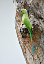
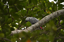
Notes:	Ring-necked parakeets (also called rose-ringed parakeets) are medium sized parrots. They are native to Africa and southern Asia.	African grey parrots have grey body feathers, black bills and red tail feathers. They are native to equatorial Africa and mostly feed on fruit, nuts and seeds with a preference for oil palm fruit.

How can you tell from Table 2 that the two organisms – the ring-necked parakeet and the African grey parrot – are closely related?

They are in the same kingdom, phylum, class, order, family and genus. They are both in the genus Psittacus but are different species: Psittacus krameri and Psittacus erithacus.

Note: Organisms can also be sorted into different life-forms which describes an organism by shape or form that reflect similarities of function rather than genetic relatedness (e.g. tree, climber/creeper, shrub).

Sampling vegetation

It is often impractical to measure all of any population of variables. For example, to count every plant of every species in a grassland would be too time-consuming, so, a sample (or subset) is measured. The aim of sampling is to select a sample which is representative of the population. Samples should be taken either at random or in a manner that allows every member of a population an equal chance of being selected without bias.

You can use random sampling with quadrats to investigate plant species within a habitat. A quadrat is a frame (usually square) used to outline a sample area for study. You can then identify and count the species present in the quadrat. There are many different sizes and types of quadrat: a suitable quadrat for short grassland vegetation would be 1 m x 1 m.

You can investigate the biodiversity of a habitat or area by looking at species richness, which is a measure of the number of different species present in an area. To do this, you could set out quadrats and count the number of species present in each quadrat and then work out an average (mean) species richness for the area.

A student investigating the species richness of a grassland set out 10 quadrats randomly and counted the number of different species in each quadrat. Quadrat number 1 2 3 4 5 6 7 8 9 10 Number of species present 7 3 8 5 6 4 6 5 10 6 Use this data to calculate the average species richness

Average species richness =  = 6

Percentage frequency is a measure of abundance, it tells you how often a species occurs in samples. For example, if a species is found in every quadrat sampled, then it has a frequency of 100%. If it is found in 1 out of 10 quadrats, then it would have a percentage frequency of 10%. Percentage frequency therefore tells you how common a species is.

Percentage frequency = 

Previous: Lesson objectives                                                                      Next: Practical activity