1 Neoclassical economics: a very brief introduction

The emergence of neoclassical economics is often called the marginalist revolution because of the importance of concepts such as marginal utility or marginal revenue. Jevons (1871) argued that the utility or pleasure we get from an object depends on how many similar objects we already have. Marginal utility often decreases as we get more of a good. Increasing consumption can, beyond a certain point, even decrease our overall utility and well-being. He illustrated this with a famous example about water:

Water, for instance, may be roughly described as the most useful of all substances. A quarter of water per day has the high utility of saving a person from dying in a most distressing manner. Several gallons a day may possess much utility for such purposes as cooking and washing; but after an adequate supply is secured for these uses, any additional quantity is a matter of indifference. All that we can say, then, is, that water, up to a certain quantity, is indispensable; that further quantities will have various degrees of utility; but that beyond a certain point the utility appears to cease.

(Jevons, 1871, pp. 52–53)

Figure 1: How much utility we get from one more drop of water depends on how much we already have

Show description|Hide description

This is a cartoon illustration featuring two characters. On the left there is a person panting, and appears thirsty and overheated. They are thinking about a glass of water. On the right there is a person wearing a shirt with a sun symbol. They are holding an umbrella and standing in a puddle, with water dripping from the umbrella. They look grumpy and uncomfortable with the amount of water raining on them.

Figure 1: How much utility we get from one more drop of water depends on how much we already have

In neoclassical models explaining the behaviour of single agents, such as a firm or a consumer, the main assumption is that they make choices by comparing marginal benefits with marginal costs. So, for instance, to find out a consumer’s demand for a good or service, we compare the additional utility they get from an extra unit with how much this additional unit would cost them, its price. In a diagram, this would look like Figure 2.

Figure 2: Comparing marginal cost (price) with marginal benefit to determine optimal consumer demand

Show description|Hide description

Figure 2 is a diagram showing how the price (on the vertical axis) relates to quantity (on the horizontal axis). The origin from where the two axes are drawn in the bottom left corner is represented by the letter O. The main line in the diagram is a blue solid decreasing straight line (so falling from top left to bottom right), which is labelled Individual demand. This is the demand line.  Figure 2 also shows a black horizontal line set at the price level P. The point where the two lines intersect is called point A. In the vertical axis, and as mentioned above, the price level of point A is price P. In the horizontal axis, the quantity is Q subscript C.

Figure 2: Comparing marginal cost (price) with marginal benefit to determine optimal consumer demand

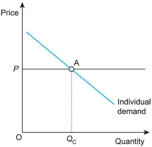
Returning to Jevons’ description of the additional benefit of an extra unit as the amount already held increases: the marginal benefit is decreasing as quantity increases. So if price is constant and provided by the market, outside the consumer’s control, the optimal individual demand for a good or service is decreasing too, reflecting the decreasing marginal utility. You can interpret the Individual demand curve as both the consumer’s demand at different prices and as the consumer’s marginal benefit from an extra unit, which determines the price they are willing to pay for it.

Activity 1: Interpreting the individual demand curve

Timing: 10 minutes

Let’s try to do the same for a firm when market price is beyond its control. This happens in a neoclassical model called perfect competition.

Assuming firms operate in the short run where at least one input to production is fixed, which means that the cost of the other inputs or factors of production rises as more are deployed, sketch a diagram of a firm’s supply curve where optimal quantity produced is set where marginal revenue equals marginal cost.

Hints:

1. The firm being a price taker in a perfectly competitive market means the marginal revenue from each product is the market price.
2. Assume that the marginal cost, the cost of making an additional unit, rises as more is produced. (In the short run, not all inputs of production can change, and there is no possibility to incorporate gains from innovation and technological progress.)

Comment

Figure 3 shows a firm’s supply in a competitive market where it is a price taker and must supply its output at the market price. Apart from an initial range of output in which increasing production improves efficiency and, therefore, marginal cost falls, the firm’s marginal cost curve is upward sloping. The horizontal line at price P also represents the marginal revenue curve, This is also the firm’s average revenue, as the price doesn’t change when it raises or lowers output.

Figure 3: Short run supply curve of a firm in a perfectly competitive market

Show description|Hide description

Figure 3 is a diagram showing how the price and cost (on the vertical axis) relate to quantity (on the horizontal axis). The origin from where the two axes are drawn in the bottom left corner is represented by the letter O. The main line in the diagram is a blue solid curve which is decreasing for very low quantities, reaches a minimum, and shoots off thereafter. The larger the quantity, the larger the increment in cost per a fixed increase in quantity. This is the marginal cost curve Figure 3 also shows a black horizontal line set at the price level P. The point where the two lines intersect is called point B. In the vertical axis, and as mentioned above, the price level of point B is price P. In the horizontal axis, the quantity is Q subscript F.

Figure 3: Short run supply curve of a firm in a perfectly competitive market

The firm maximises profit at point B, producing quantity Q_F. If production is below Q_F, price (the firm’s marginal revenue in perfect competition) is higher than marginal cost, so the firm can earn more profit by expanding production until marginal cost and marginal revenue (price) are equal. If production is above Q_F, price is lower than marginal cost, and the firm incurs a loss for the last unit produced; so it should reduce production until marginal cost and marginal revenue (price) are equal. The marginal cost curve is also the firm’s supply curve when operating in perfect competition.

While this activity used a short run model of the firm, the long run model would be very similar. Even though in the long run all inputs of production can change, the most common assumption is that marginal costs increase, and increase by more the higher the quantity due to physical and mental limits of machines, workers, and inputs in general.