Golden Globe Ocean Race: Global Biodiversity

The Discovery of Biodiversity

Today we take it as read that there are some places on Earth that contain more types of organisms than others. Placing a photograph of Greenland next to a photograph of central America for example would immediately contrast a cold and relatively barren region with richly tropical bioscope (Figure 1). However, such information was not always public knowledge and it wasn’t until the nineteenth and early twentieth centuries, when naturalists began making regular exploratory voyages to the far corners of the globe, that the first scientific observations of how biodiversity varies over the face of the Earth were made.

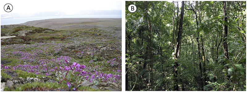Figure 1. Field photographs of the vegetation growing in Jamesonland, East Greenland (A), and Barro Colorado Island, Panama (B).

Describing the extraordinary diversity of plant life in a tropical rainforest, for example, Alfred Russell Wallace wrote of "the parasitic plants growing on the trunks and branches, the wonderful variety of the foliage, the strange fruits and seeds that lie rotting on the ground" (Wallace 1909). In an account of his expedition to South America, Alexander von Humboldt (pictured in Figure 2) commented that "there, the different climates are ranged the one above the other, stage by stage, like the vegetable zones, whose succession they limit" (von Humboldt 1845–1858).

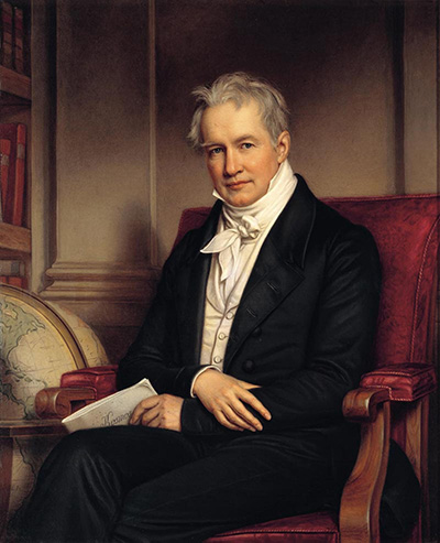Figure 2. A portrait of Alexander von Humboldt. Although the language used by Wallace and Humboldt is somewhat out-of-date, the observations they made were revolutionary in their detail as well as their scope. Humboldt in particular was a great traveller and from 1799 to 1804 he explored Venezuela, the Andes, Mexico, Tenerife, Cuba and the United States together with the botanist Aimé Bonpland (Jackson 2009). The specimens collected during these trips were numerous and diverse, ranging from plants to geological specimens, but crucially they were accompanied by precise records of their geographic location together with measurements of the atmospheric and geophysical conditions, such as temperature and elevation, at each location.

When Humboldt returned home to write up the results of what he had seen and collected during his voyages the first text he produced was entitled Essay on the Geography of Plants (Humboldt 1807). In this book Humboldt set out his vision of a world in which the Earth surface, the oceans, the atmosphere, and the creatures living in them, were intimately connected in what he called a “general physics of the Earth”. Key to this idea of a “unity of nature” was the geographical link between the organisms and specimens that had been collected, and the measurements of the physical world that had been made with instrumentation.

A focus on geography required him to develop new techniques, such as isotherms, for displaying his observations and they allowed him to recognise patterns in the data he had collected. In doing so, Humboldt turned his back on the prevalent religious explanations for phenomena seen in nature and instead sought process-based scientific explanations for the patterns he saw in his observations. Such a quantitative approach allowed him to investigate how Earth’s surface temperature varies with height, how heat and material is transported by winds and ocean currents, as well as how latitude affects the snowline of mountains (Jackson 2009). He interpreted his biological data in light of the physical measurements he made in order to make novel and bold statements about the factors that control the distribution of life on Earth, and as an example, in his Essay on the Geography of Plants Humboldt highlighted that local environmental conditions are frequently a better predictor of plant form than their evolutionary relationships (Humboldt 1807).  

To Humboldt, then, should go the credit for founding a large part of what we know today as the discipline of biogeography. This discipline involves the systematic study of biodiversity and ecosystems in geographical space and through geological time, and it is the focus of this Ocean Race Topic. We first look at how biodiversity is measured and why it is important to us as human beings, before examining a first-order pattern in the distribution of biodiversity on Earth and evaluating hypotheses that have been proposed to explain it. We then revisit the course taken by the Golden Globe sailors, and by looking again at the voyage made by own sailor Antoine Cousot, we investigate the biodiversity of islands, which are special and often threatened havens for life on Earth. We finish by considering the future of biodiversity from a geographical perspective.

The Measurement and Importance of Biodiversity

Biodiversity in its broadest sense refers to the diversity of living things. There are several different ways to measure biodiversity and each quantifies a slightly different aspect of biological variety. Perhaps the simplest and most intuitive measure of biodiversity is morphological diversity. Sometimes we look at organisms without knowing what they called but we can recognise that they have different visual appearances. Birds are an example that you may have come across. Quite often we look into the garden or into a field and see a number of birds feeding or moving through a hedgerow. Some of these we recognise and instantly name: a blackbird, a robin, a blue tit and so on. However, some birds only visit particular countries or regions at certain times of the year, and classic examples are the fieldfare (Turdus pilaris) that is a winter migrant to the UK as a whole, and the avocet (Recurvirostra avosetta) that lives in the east of the UK all year round but flocks to the southwest of the UK in winter. Since these winter migrants are not seen so regularly, their names are often not very familiar to us. However, when these birds arrive we are able to see that they have different visual appearances to the birds we are used to—the blue-grey back and the brown wings of the fieldfare, and the long upturned beak of the white and black avocet—and this allows to us to recognise a change in the morphological diversity of the birds that we see.

Another way to measure biodiversity is to think about the ways in which different organisms live. For instance, some organisms make food using the light of the sun (they are photosynthetic), others eat plants (they are herbivores) while some only eat other animals (they are predators). Feeding habit is one way to partition organisms into different groups, but there are several other things that can also be used. How does the organism move? Where does it live? How does it reproduce? What is its lifespan? Taken together, such factors can be used to place organisms into groups based on their ecological function. Doing this for particular groups of organisms or for particular regions allows for the measurement of functional diversity. For example, if a field contains a cow, a sheep and a kangaroo, we can instantly say that there are three different organisms in the field because they each look very different to one another. However, each of these organisms feeds by grazing, and so from the perspective of feeding habit there is just a single functional type in the field.

We have already used names in our discussion of morphological and functional diversity, and these names are the root of a third measure of biodiversity: taxonomic diversity. Organisms are all given names, and these names have two parts. Humans are known as Homo sapiens, and as we have seen the fieldfare is called Turdus pilaris while the avocet is called Recurvirostra avosetta. The first of these names, Homo for example, is the genus to which an organism belongs, while the second of these names, in this case sapiens, is the species to which an organism belongs. Genus and species are part of wider system of classification known as the taxonomic hierarchy. For humans, this hierarchy is as follows:

• Kingdom – Animalia
• Phylum – Chordata
• Class – Mammalia
• Order – Primates
• Family – Hominidae
• Genus – Homo
• Species – sapiens

Each of these different levels has certain distinguishing features. The phylum Chordata contains organisms with a spinal cord, the Class Mammalia (the mammals) contains organisms that nourish their offspring with milk produced in the mammary glands of the mother, while the Family Hominidae contains organisms that walk upright. The basic unit of the taxonomic hierarchy is the species, and when scientists discuss diversity they often mean the number of species, which is termed species richness. In principle it is possible to go to any region of the world and, given the right books and taxonomic training, count the number of species that are living there. 

However, why would anyone want to do this? Why is biodiversity in any of its forms useful or important to us? The first thing to note is that organisms live within ecosystems, and these organisms play a role in the function of ecosystems. There are four broad categories of ecosystem function:

(1) Regulating functions, such as the transport, storage and recycling of nutrients.

(2) Supporting functions, such as the provision of suitable living spaces for biotic communities and individual species.

(3) Provisioning functions, such as the production of raw materials that are used for any purpose other than food.

(4) Cultural functions, such as the extent and variety of natural landscapes.

Humans exploit these ecosystem functions, which have a monetary as well a non-material benefit to society. For example, humans rely on ecosystem functions for the provision of food and nutrition, while tourism is enhanced in areas of outstanding natural beauty that are also able to provide opportunities for reflection and recreation (Christie et al. 2012). Many such ecosystem functions are enhanced by increased species richness, and case studies using plants, bacteria and aquatic plants such as seagrass have all shown that the probability of an ecosystem sustaining its overall function increases as species richness increases (Gamfeldt et al. 2008). It is therefore imperative that we take care of biodiversity because it has a positive effect on the function of ecosystems that we rely upon in our daily lives.

Establishing Patterns and Proposing Hypotheses

Owing to the importance of biodiversity for humanity as a whole, as well as an academic interest in why biodiversity is not uniform across the globe, scientists have built on the pioneering efforts of Humboldt and gathered data on the species richness of almost all ecosystems from the tropics to the poles. These data show that tropical regions generally contain more species than regions at higher latitudes. Certain areas such as the high Arctic and the interior of the Sahara Desert are characterized by very low richness (<100 species per 10,000km2), whereas others such as tropical rainforests contain extraordinarily high richness (>5000 species per 10,000km2). This pattern is highlighted in Figure 3, which shows the number of tree species found in three biomes situated on a latitudinal transect from low latitudes close to the equator (tropical biome) to to high latitudes near the poles (boreal biome).

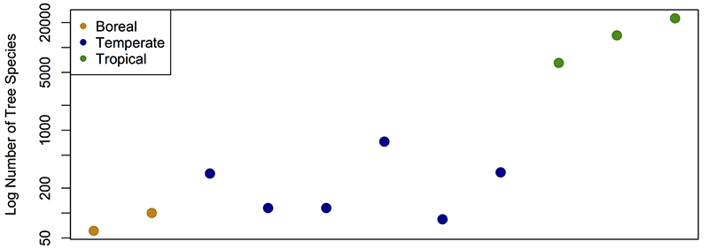Figure 3. The number of tree species in three of the world's major biomes. Tropical biome = between 23.5 degrees north and south of the equator. Temperate biome = between 23.5 degrees and 50 degrees north and south of the equator. Boreal biome = between 50 degrees and 70 degrees north and south of the equator. Note that the number of species is plotted on a logarithmic scale. Data from Fine and Ree (2006).

This pattern is pervasive, and characterises groups ranging from the vascular plants shown as an example in Figure 3, to marine molluscs such as bivalves, as well as higher vertebrates such as lizards and salamanders. Owing to its ubiquity it is known as the latitudinal diversity gradient (LDG). However, despite the importance of the LDG as a first-order feature of the biosphere, researchers have so far been unable to come up with single convincing explanation for it. To date, scientific research has focussed on testing the following four central hypotheses to explain the LDG:

(1) Habitat heterogeneity may control the diversity gradients in an area by influencing the composition of different communities

(2) In general, the species richness of a region is strongly associated with its present-day climate. For plants, it has been suggested that the geographical patterns of plant species richness are dependent on the amount of heat and water that is available to plants.

(3) Regional differences in species richness may also be explained by contrasting regional geological and climatic histories. These include climatic change associated with the waxing and waning of ice sheets during the last 2.6 million years, as well as tectonic events such as the uplift of mountains.

(4) Random placement of species geographic ranges on a bounded map (the world) produces a peak in species richness near the centre of the domain, and such geometric effects may explain regional–global richness gradients.  

Hypotheses (1) (2) and (3) each clearly hark back to the work of Humboldt because they rely on the geographic linkage between biology, in this case species richness, and data on the physical properties of the world. However, the lack of scientific consensus on the exact cause of the LDG is problematic because it means that we do not fully understand the mechanisms responsible for the geographic variation in species richness. It also means that scientists are unable to fully predict, and hence mitigate, the ecological effects of the current climate and biodiversity crises, which threaten species-rich tropical ecosystems and the critical functions that they provide.

Ocean Racing and Global Biodiversity

The sailors in the Golden Globe Race 2018 began their voyages in Les Sables-d’Olonne in France, which sits at 46.49 degrees north. On the outward portion of the race the sailors made their way south across the Bay of Biscay, down the Atlantic Ocean and crossing the equator, before rounding the Cape of Good Hope on the southern tip of Africa at 34.36 degrees south (Figure 4). On this outward Atlantic leg, once the sailors left the Mediterranean behind and headed south, their boats would have been propelled past the east coast of north Africa by the trade winds. This represents the start of a latitudinal transect that is truly extraordinary from a biogeographic perspective. To begin with the sailors passed the Sahara Desert, which is characterised by extremely low diversity and populated by plants and animals adapted to hot days, cold nights, and extremely low rainfall. 

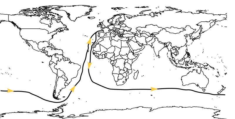Figure 4. Map of the world with the 2018 Golden Globe Race routes superimposed as a solid black line with yellow arrows indicating sailing direction.

Next, they sailed past the grasslands and savannahs of the Sahel and Sudan. These zones are home to many species of grass, which coexist with trees that form woodlands in a balance that is thought to be regulated in a large part by fire. In particular, the expansion of grasslands and savannahs is promoted by frequent fires that burn using grasses as fuel and which prevent the establishment of woodlands. In contrast, once a woodland becomes established, the dense tree cover prevents the growth of grasses and creates a cool and humid microclimate that prevents large fires. These grasslands and savannahs are extraordinarily dynamic places, and an example of the phenomena that can be seen in this region of the world is the formation of vegetation into patterns in certain dryland ecosystems (Figure 5). It is thought that such vegetation patterns result from the enhanced infiltration of water into vegetated ground compared with bare ground which promote the growth of vegetation at very local scales but inhibit vegetation growth over a larger area because of competition for water (Mander et al. 2017). If you have Google Earth, you can explore these vegetation patterns for yourself at the following co-ordinates:

Spots – 11°34′ 27.91′′ N, 27°56′ 19.72′′ E

Labyrinths – 11°17′ 16.24′′ N, 27°59′ 29.92′′ E

Gaps – 10°59′ 25.85′′ N, 28°15′ 28.19′′ E

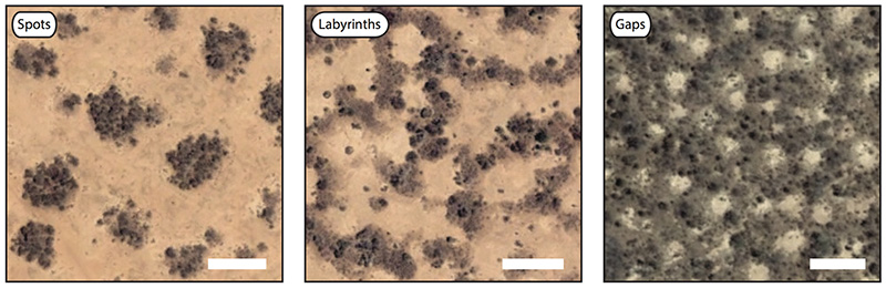Figure 5. Satellite images of vegetation organised into intricate patterns in South Sudan. Scale bars represent 50 metres. Adapted from Mander et al. (2017).

Once past these semi-arid parts of the African continent the sailors entered the equatorial region and passed the two principal blocks of tropical rainforest in West Africa. The first is the Guinea rainforest block, which stretches from Guinea and Sierra Leone through the Ivory Coast to Ghana, and the second is the Cameroon–Gabon rainforest block, which extends from Nigeria through Cameroon and Gabon into the Congo. The rainforests of the Cameroon–Gabon block are the second largest block of rainforests in the world after the rainforests of the Amazon, and they are separated from the Guinea rainforest block by a corridor of savannah in Benin and Togo known as the Dahomey Gap. By sailing this transect, from the Sahara all the way south to equatorial West Africa, the Golden Globe sailors have made an almost perfect traverse through the LDG.

After making their way through the Atlantic Ocean, the Golden Globe sailors rounded the Cape of Good Hope on the southern tip of Africa. In doing so they passed an extraordinary exception to the LDG: the Cape Flora. Situated in temperate latitudes in a Mediterranean climate, the Cape Flora is a biodiversity hotspot that amounts to around 9,000 species in an area of 90,000 km2 ­(Linder 2005). This level of diversity is unique among plants at temperate latitudes and is comparable to the diversity of plants found in tropical rainforests. Plant groups that are typical elements of the Cape Flora today appear gradually in the geological record, and it is thought that their spread was facilitated by climatic changes associated with the evolution of the Benguela current and upwelling system in southern West Africa. The exceptionally high diversity of the Cape Flora may also have been enhanced by modified fire regimes, or by pollinator and habitat specialization.

The Biodiversity of Islands

The Cape Flora also contains a very high number of endemic species (~70%). Endemic species are species that only live in one geographical region, and in this respect the Cape Flora has levels of endemism that are more characteristic of islands such as Hawaii or Madagascar than a continental area (Linder 2005). Our own intrepid sailor Antoine Cousot stopped at the Canary Islands and passed the Cape Verde Islands on his voyage from France to Brazil, and the Golden Globe Race mentions Prince Edward Island, the Crozet Islands, the Kergulen Islands, Snares Islands, and the Bounty Islands in the sailing directions for its 2018 race.

Indeed, if you examine Figure 4 again, you can see that the land surface on which plants and animals live can be divided into two broad categories: islands and the mainland. Islands have long-fascinated biogeographers because they are intrinsically appealing objects to study; they are simpler than a whole continent or ocean and are visibly discrete objects that have clear boundaries (MacArthur and Wilson 1967). As a result of their discrete and bounded nature, scientists interested in the species that live on islands can also harbour a realistic hope that an island’s biota can be assessed with a degree of completeness. One of the most striking features of islands is the consistent relationship between the area of an island and the number of species it contains (Figure 6).

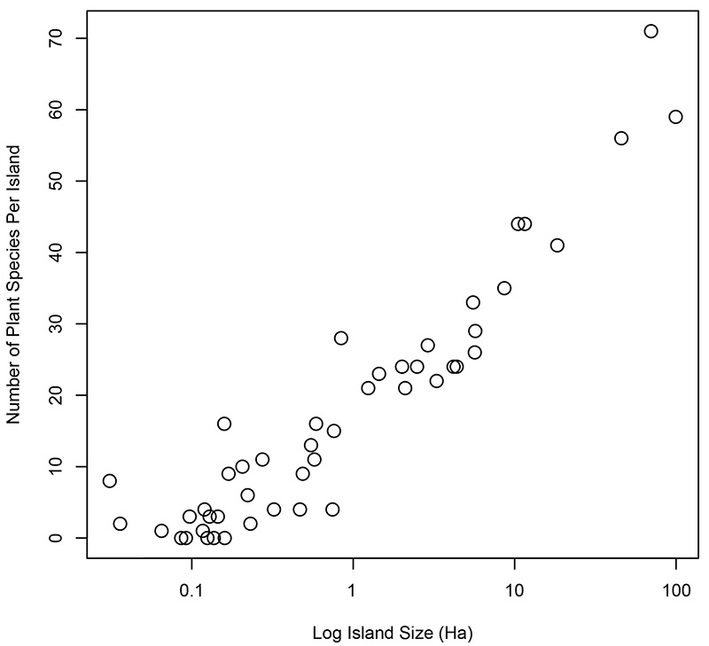Figure 6. The number of plant species on islands of different sizes. Data were collected by Kohn and Walsh (1994) from the Shetland Islands, UK, and have been re-plotted here.

This relationship is known as the species-area relationship and it has been replicated many times in different islands across the world. It is a hugely important relationship today because many of the world’s species that are at the greatest risk of extinction due to climate change and destructive human activities are endemic to small islands. Endemic species are at high risk of extinction because their geographic range is often extremely small, their population size is typically low, and they are also often poorly equipped to deal with invasive predators such as rodents and cats that are frequently introduced to islands by humans.

Human activity is in the process of creating islands by the process of habitat fragmentation. Forests that were once continuous across great tracts of land are now reduced to isolated patches hundreds of miles apart. In the temperate latitudes the interstices between forests patches are often farmland that is used to grow crops that we consume directly, or indirectly though livestock, and in the tropics it is commercial logging that breaks rainforests into isolated fragments. If threatened species are to survive into the future, it is vital that scientists fully understand the mechanisms that underpin why species richness varies geographically. The research being done in this area relies on Humboldt’s insistence of linking collections of organisms and specimens to precise measurements of the physical world, and preventing the irreversible loss of global biodiversity will require us to pursue his vision of a “unity of nature”.