1 How likely are particular results?

In real experiments, as opposed to hypothetical ones, it is very rare that scientists make a sufficiently large number of measurements to obtain a smooth continuous distribution like that shown in Figure 1.

Figure 1 Distribution for repeated measurements of the unit cell constant of a batch of industrial catalyst.

Show description|Hide description

Distribution for repeated measurements of the unit cell constant of a batch of industrial catalyst shgown in a graph. The left axis is ‘number of measurements’ and the bottom axis is ‘cell constant/nm.

Figure 1 Distribution for repeated measurements of the unit cell constant of a batch of industrial catalyst.

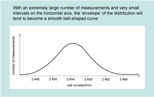
However, it is often convenient to assume a particular mathematical form for typically distributed measurements, and the form that is usually assumed is the normal distribution , so-called because it is very common in nature. The normal distribution corresponds to a bell-shaped curve which is symmetric about its peak, as illustrated in Figure 1. Repeated independent measurements of the same quantity (such as the breadth of an object, or its mass) approximate to a normal distribution. The more data are collected, the closer they will come to describing a normal distribution curve.

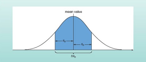
The peak of the normal distribution curve corresponds to the mean value of the distribution, as shown in Figure 2. This figure also illustrates how the standard deviation of a set of measurements is related to the spread. Although it is beyond the scope of this course to prove this, the area under a portion of a distribution curve within a certain range represents the number of measurements that lie within that range, as a proportion of the whole set. For a normal distribution, it turns out that 68% of the measurements lie within one standard deviation (i.e. within ±s_n) of the mean value. Conversely, 32% of the measurements will lie outside this range. If you make a single additional measurement, it is therefore just over twice as probable that this one measurement will fall within one standard deviation of the mean than that it will fall outside this range. For a normal distribution, it also turns out that 95% of measurements are likely to fall within two standard deviations of the mean and 99.7% within three standard deviations of the mean.

Figure 2 The shaded area under this normal distribution curve represents the measurements that lie within one standard deviation of the mean. This area is 68% of the total area under the curve, so 68% of the measurements are expected to fall within this range.

Show description|Hide description

Figure 2 The shaded area under this normal distribution curve represents the measurements that lie within one standard deviation of the mean. This area is 68% of the total area under the curve, so 68% of the measurements are expected to fall within this range.

Figure 2 The shaded area under this normal distribution curve represents the measurements that lie within one standard deviation of the ...

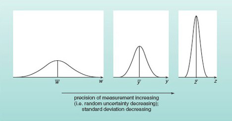
Remembering that precise measurements were defined in Week 7 [Tip: hold Ctrl and click a link to open it in a new tab. (Hide tip)]   as those for which the scatter was small, you will appreciate that the more precise a repeated set of the same number of measurements of a particular quantity, the more highly peaked the distribution curve and the smaller the standard deviation will be. A very broad distribution on the other hand, corresponds to measurements with considerable scatter and the standard deviation will be large. These trends are illustrated in Figure 3.

Figure 3 Normal distribution curves for three independent sets of measurements, with the same number of measurements in each set. The measurements of quantity w are subject to large random uncertainties, while those of quantity y are more precise and those of z more precise still.

Show description|Hide description

Figure 3 Normal distribution curves for three independent sets of measurements, with the same number of measurements in each set. The measurements of quantity w are subject to large random uncertainties, while those of quantity y are more precise and those of z more precise still.

Figure 3 Normal distribution curves for three independent sets of measurements, with the same number of measurements in each set. The ...