Find out more about The Open University's Statistics courses and qualifications.

In statistics, analysis is often presented as beginning with data. In practice, this is rarely true. Before any data is collected, there are already expectations about what values are plausible, which outcomes seem unlikely, and what patterns might emerge. These expectations arise from previous studies, theoretical understanding, and practical experience.

In many real-world problems, data alone is not sufficient. This is particularly evident in early clinical studies, where only a small number of patients may be observed, or in climate science, where predictions must be made using incomplete information about the future. The key question is therefore not whether prior knowledge exists, but whether we choose to recognise and incorporate it meaningfully.

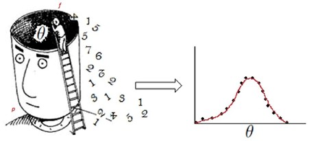
Figure 1 Conceptual illustration of prior elicitation, where expert knowledge about an unknown parameter is translated into a probability distribution

A simple introduction to Bayesian thinking

Bayesian statistics provides a framework for combining prior knowledge with observed data. Named after Thomas Bayes, an eighteenth-century mathematician, this approach is based on a simple idea: our beliefs about an unknown quantity can be updated as new evidence becomes available.

Rather than eliminating uncertainty, Bayesian methods quantify it using probability. The process begins with a prior distribution, representing beliefs before observing the data. The likelihood captures the information from the observed data. These are combined to produce the posterior distribution, which reflects updated beliefs after considering the evidence.

Why prior knowledge matters

Prior knowledge becomes particularly important when data is limited. This situation arises frequently in applied settings. For example, early-stage clinical trials often involve small sample sizes, while environmental and climate research must rely on incomplete and evolving data.

At the same time, experts often possess valuable domain knowledge. A clinician may draw on experience with similar treatments, while a climate scientist may understand long-term physical patterns and constraints. Even when experts cannot provide precise numerical answers, they can often describe what values are realistic and what outcomes are unlikely. If such knowledge is ignored, it does not disappear – it simply remains informal and unexamined.

From expert opinion to a statistical prior

A central challenge in Bayesian modelling is constructing the prior distribution. This is where prior elicitation plays a crucial role. Prior elicitation is the process of translating expert knowledge into a probability distribution that can be formally incorporated into a statistical model.

In my PhD research in Statistics, I work on prior elicitation and develop interactive software tools that help experts express their beliefs in a structured way. These tools guide experts in expressing their beliefs in a structured way, without requiring advanced statistical knowledge.

Rather than asking experts for a single number, elicitation focuses on uncertainty. Experts are often more comfortable describing ranges, identifying values that seem unlikely or indicating where they think the true value is most likely to lie.

A simple illustration

Consider estimating the probability of a side effect for a new medical treatment when only limited data is available. Instead of asking for a single number, a clinician might be asked to provide three values:

• A lower value, below which the probability is unlikely to fall (e.g. the 25th percentile)
• A central value representing their best estimate (e.g. the median)
• An upper value, above which the probability is unlikely to rise (e.g. the 75th percentile).

These summaries are intuitive and capture uncertainty more effectively than a single estimate.

Suppose the clinician suggests that the probability is unlikely to be below 0.35, most likely around 0.4, and unlikely to exceed 0.45. These values can be used to construct a prior distribution, using a specific form of probability distributions called the Beta distribution.

Now consider data from a small study, where 12 out of 40 patients experience the side effect. The observed proportion is 0.30, which would be the classical estimate.

In the Bayesian framework, this data is combined with the prior to produce a posterior distribution. The resulting estimate reflects both sources of information. In this case, the posterior mean is around 0.35, lying between the prior (centred near 0.4) and the observed data (0.3). This demonstrates how Bayesian updating works: the estimate shifts from prior beliefs toward the data (see Figure 2).

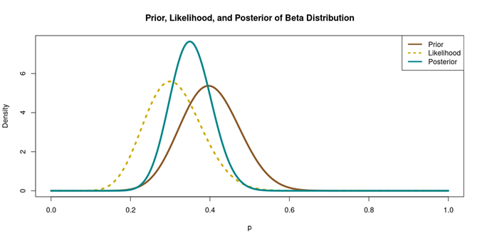
Figure 2 Illustration of Bayesian updating showing prior, likelihood, and posterior distributionsShow description Visual representation of how a probability distribution is updated with new evidence using Bayesian inference. Specifically, it plots the Prior, Likelihood, and Posterior for a Beta distribution. X-Axis (p): Represents the probability parameter p, ranging from 0.0 to 1.0. Y-Axis: Measures the probability density, ranging from 0 to 6+. The prior curve is a relatively wide distribution centered near 0.4. The likelihood curve peaks earlier, around 0.3. The posterior curve is taller and narrower than the other two. It peaks around 0.35.

In conclusion, Bayesian statistics represents a broader way of thinking about learning from data. Prior elicitation plays a key role in this process by connecting expert judgement with formal statistical inference. By incorporating expert knowledge in a structured and transparent way, Bayesian methods allow us to make better use of limited data while acknowledging uncertainty.