It’s just over a year since I became a Lecturer In Environmental Sciences in the Department of Environment, Earth and Ecosystems, but I already feel very at home at the Open University. Thank you for reading my first article here on OpenLearn.
I’m part of a team of British and French scientists with a new study published in Nature about Antarctic ice sheet instability. Here is a Guardian article I wrote as an introduction to our work. I also recorded a video explaining our focus on Antarctica and the uncertainty surrounding the impact of global warming. Following the video is a slightly more in depth description of our recent research findings.
Unstable ice sheets
The idea that parts of the Antarctic ice sheet could become “unstable” goes back four decades. In the 1970s two US material scientists who had become interested in glacial ice, Terry Hughes and Hans Weertman, and US-based British glaciologist John Mercer were among those to propose that the parts of the ice sheet resting on bedrock below sea level might be vulnerable to a mechanism of self-sustaining ice loss they called “Marine Ice Sheet Instability”, or MISI.
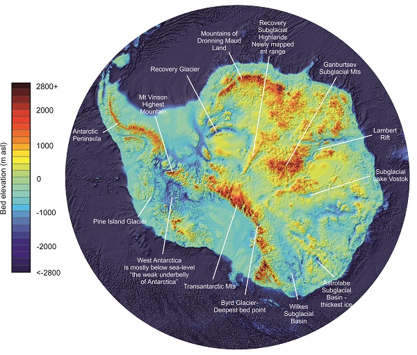
 Bedmap2 bedrock topography map (Fretwell et al., 2013) with some points of interest.
Above is a map from the latest measurements of Antarctic bedrock topography. Blue-green colours are below sea level. You can see the broad outline of the continental shelf, with a steep edge falling off to the dark blue deep ocean. This BBC article has a lovely fly-over video, bringing to life the world of great mountain ranges and deep troughs beneath the ice.
Around three quarters of the West Antarctic ice sheet has an underwater bed, with a potential contribution to global sea level rise of over three metres, and as you can see parts of East Antarctica are also marine. In other words, some serious amounts of sea level rise. But how likely is this instability? And how fast would it happen?
Retreating boundaries
If the boundary between floating ice shelves and ice resting on bedrock – the ‘grounding line’ – retreats inland, the ice losses contribute to sea level rise. The grounding line can begin to retreat if warm ocean water rapidly melts the ice, or if an ice shelf is damaged or collapses (because the ice flowing into that region speeds up).
The idea behind marine ice sheet instability is that thicker ice tends to flows faster. So if the grounding line retreats along bedrock that slopes downwards from the coast, the thickness of the ice at the grounding line increases. This tends to make the ice flow faster, which makes the grounding line retreat further inland… and so on. In other words this is a positive feedback, and ice losses are sustained until the grounding line finds a new stable position such as a flatter area of bedrock.
Last year satellite data confirmed that the grounding line in the Amundsen Sea Embayment in West Antarctica is showing sustained and widespread retreat, and two modelling studies of the great Pine Island Glacier (shown on the map) and next door Thwaites Glacier predicted this retreat is indeed unstable, driven by warm “Circumpolar Deep Water” coming onto the continental shelf. It’s hard to say whether human-caused climate change made this particular ocean circulation pattern more likely: it’s possible, but not confirmed.
So what next? Will this retreat continue? Will it start elsewhere on the continent? We’ve already seen some ice shelves collapse on the Antarctic Peninsula and others around the continent might collapse in future. Some ocean models have also predicted warmer waters around the coastline in future, including new intrusions of Circumpolar Deep Water on the continental shelf.
Predicting the future
Unfortunately “MISI” isn't, er, “easy” to simulate with computer models because you need to do the calculations on a very fine spatial scale, as I wrote about here. This makes the models very computationally expensive (i.e. slow!). The two studies last year coped with this by only simulating a small region of Antarctica. So far we haven’t yet seen this level of detail for the whole continent.
The alternative, then, is to use a computer model with a coarser resolution – bigger pixels, if you like – with more simplifications.
Some previous predictions for Antarctic ice sheet instability used these coarser models. Others didn’t use a computer model at all, but combinations of expert judgement and extrapolation of past observations into the future. When the IPCC made its latest assessment in 2013, they didn’t think these studies were strong enough evidence to make a statement about the potential for sea level rise from instability. They only said it would not be more than “several tenths of a metre”.
We predict that Antarctic ice sheet instability will most likely contribute 10 cm to sea level rise by 2100, and is extremely unlikely (a 1 in 20 chance) of exceeding 30 cm, under a mid-high climate scenario called A1B. Our upper limit of 30 cm is quite a lot lower than those simpler studies, of which some predicted half a metre to a metre of sea level rise from MISI. So our results generated some news headlines (by the way we never said “exaggerated” in that last link, but how the media reports science is a whole other story…) and good blog posts.
But I want to talk here about the process, the way we made our predictions.
How reliable are models?
Our study has two new elements. The first is that we try to make a thorough assessment of the model uncertainty: how different can the results be, if we twiddle the simplifications and inputs a bit? We used three thousand versions of the model to make our predictions from the recent past to the year 2200. Each had different versions of the physical laws governing how ice sliding depends on the bed (such as how slippery it is), different maps of the bedrock topography, and different dates of the triggering of instability by warm ocean water or ice shelf collapse. This approach of using a whole ‘ensemble’ of simulations is very common in climate science and other areas of science that use computer models.
The ensemble gives us our first, or “prior”, prediction for sea level rise in the future, given all the model uncertainties that we have included. Instead of a single prediction it is a whole distribution (like a bell curve): a range of possible futures.
Once we have our three thousand predictions: now what? We come to our second element: testing the different model versions with observations of the recent past. We compared the simulated rate of past ice losses in the Amundsen Sea Embayment with satellite observations (from the IMBIE project). Each model version then had a score from best to worst.
The scores, called “likelihoods”, gave us a measure of how reliable the model versions were. We used them to give greater weight to the “best” and less weight to the “worst” to get our final, or “posterior”, predictions. This uses a mathematical formula called Bayes’ theorem, which is often used by spam filters! It’s very common for combining information from mathematical or computer models (like spam filters) and observations (like pressing Junk or Not Junk…).
The weights have the effect of ‘squishing up’ the distribution, making it narrower – and therefore making our uncertainties in future sea level rise smaller. In fact, they made our predictions for sea level rise generally lower than the “prior” predictions from the model alone.
Using observations
That’s why we called our paper “Potential sea-level rise from Antarctic ice-sheet instability constrained by observations”. It’s a double-meaning – both that we tested our model with observations, and also that the observations reduced the predicted sea level rise.
Testing our model with observations gives us more confidence in its predictions. And the strength of the Bayesian approach is that we can estimate probabilities of different amounts of sea level rise in the future, which is important for making decisions about coastal defences.
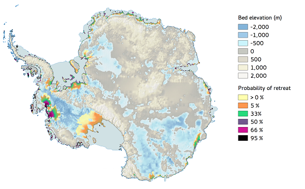
For example, the map below shows our predictions for the probability of grounding line retreat around the coastline by 2200, overlaid on the bedrock topography (where blue is below sea level). Pine Island and Thwaites Glaciers are the darkest regions, with the highest probabilities of retreat. Some areas in East Antarctica have also retreated, but we found the higher and less slippery bed meant that retreat was not that substantial. We also found that theoretical limits (in the computer model) restricted the rate at which ice could be lost. We think these are some of the reasons why our results were lower than some previous studies.
 Predicted probability of grounding line retreat by 2200 (Ritz et al., Nature, 2015), overlaid on bedrock topography map (Le Brocq et al., 2010).
So the strengths of our study are that we use a computer model (instead of expert judgement and extrapolation), that we test it with observations, and that we use Bayes’ theorem to estimate probabilities of sea level rise.
Limitations
But there always limitations, and these are important to bear in mind too. Our model has simplifications to make the calculations faster. So even though we did try to assess its uncertainties and test it with observations we’d rather have more detailed calculations instead. This is only now becoming possible with more computing power.
Even testing with observations has some built in assumptions. A model that is good at simulating the recent past isn’t guaranteed to be good at predicting the future. Success at reproducing the observations is, one could say, necessary but not sufficient. It’s the least we can do.
And finally, our knowledge always has bounds. The natural world has a habit of surprising us. This study uses our current understanding of known physical theories about how ice behaves, and our current observations from the Amundsen Sea Embayment. In time we will improve our understanding and measurements and make predictions again. These might confirm our study, or they might find something new.
Science is an ever-evolving process. And that’s what makes it so exciting.
Want to find out more?
Listen to Tamsin Edwards speak about her research on the OU/BBC radio programme, Inside Science, read articles from the Climate News Network, or to take your interest further, try a free course or look into studying Environmental Science at the Open University.


Rate and Review
Rate this video
Review this video
Log into OpenLearn to leave reviews and join in the conversation.
Video reviews