3.7 Analytical notation

An analysis set out on several levels, such as that given in Example 18a–d, is one way of demonstrating some linear progressions and hidden patterns underlying the musical surface. This is rather unwieldy, however, especially when it comes to analysing longer sections of music. What we need is a way of showing these levels clearly and succinctly all on a single pair of staves. This is the reason for the development of analytical notation.

The notation used to assemble voice-leading graphs was originally evolved by Schenker in the 1920s and 1930s, and has been extended since. Some of Schenker's symbols have already been used in this course: the use of ‘P’ and ‘N’ to label passing notes and neighbour notes respectively; the use of figures such as ‘10–10–10’ to indicate interval patterns; the use of crossing straight lines to show a voice exchange. What is needed, in addition to labels of this sort, is a method of indicating a hierarchy between notes, without having to write them out on several different levels as you did at the end of the video activity. The way that analytical notation achieves this is by the use of some ordinary musical symbols: noteheads, stems, and slurs.

In an analytical foreground graph, showing insights such as those we have been studying in this course, these symbols have the meanings listed below.

• Noteheads are used for all the notes that the graph wants to analyse. This means that, in comparison with the score, some notes may be missed out – either because they are very local elaborations (grace notes and the like), or because the graph chooses to concentrate on other voices in the harmony (many graphs analyse only the bass and the treble, and miss out inner parts).

• Stems are added to noteheads to indicate locally consonant notes. In other words, bass notes and treble notes that form consonant harmonies with each other each receive stems and may often be aligned one above the other (even if they are not literally simultaneous in the score). Stemmed noteheads look like crotchets, of course: but in an analytical graph, this indicates structural importance, and not rhythm or duration in time.

• Slurs are used to show the relationship of unstemmed noteheads to the stemmed notes. This relationship will generally be one of the cases discussed in Sections 3.3 and 3.4: the unstemmed note will be a passing note, neighbour note, or part of an arpeggiation, and a slur will connect it to the consonant note with which it belongs.

One further piece of explanation at this stage: because the use of noteheads, stems and slurs can make even a simple graph look cluttered very quickly, analytical graphs often miss out bar lines altogether. To enable you to keep track of the relationship between the graph and the score, bar numbers are included above the graph at strategic points.

If you keep these rules in mind, you should be able to make sense of any voice-leading graph, although these can look daunting at first. I now want you to try interpreting graphs of the two passages you have spent most time with in this course.

Activity 20

Examples 19 and 20 show foreground graphs of Sonata K545, first movement, bars 1–8 and Sonata K570, last movement, bars 1–4, respectively. Compare the graphs with their related scores by clicking on the link below immediately before Example 19. Refer to the explanations above of the meaning of the symbols used. In each case, write notes answering the following questions.

1. What does the graph tell us about the structure of the music?

2. What are the deepest-level events in this extract, and how are they shown in the graph?

3. What types of prolongation (i.e. neighbour notes, passing notes, suspension, arpeggiation) are used to transform the skeletal model into the musical surface?

Click to view a pdf of the scores [Tip: hold Ctrl and click a link to open it in a new tab. (Hide tip)] .

Maximise

Example 19 Mozart, Piano Sonata in C, K545, first movement, bars 1–8: foreground analysis

Maximise

Example 20 Mozart, Piano Sonata in B flat, K570, last movement, bars 1–4: foreground analysis

Discussion

I hope that you can see how Example 20 tries to represent many of the things brought out by the four levels of Example 18 (which you saw explained in the video). Your answers to the questions above may have included the following points.

• Each of these graphs suggests that the music is structured hierarchically, in the way described throughout this course.

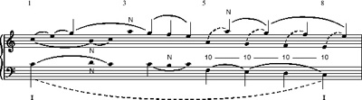
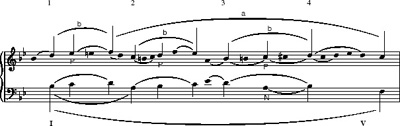
• The deepest levels analysed in each graph are those indicated by the longest slurs. In Example 19, the longest slur (shown as a broken slur – more on this later) connects the first and last notes, which both support tonic chords of C major. In Example 20, the longest slur also connects the first and last bass notes. Another long slur in the top lines, marked ‘a’, links together the F of bar 1 and the C at the end, to show that the melody line moves in a linear progression from the first of these notes, by step, to the other. Roman numerals have been added to make the overall progression in each graph clearer.

• In both graphs, the symbols ‘N’ and ‘P’ have been used to show some passing notes and neighbour notes. Slurs within slurs have been used to show how harmonic lines are nested inside each other.

Example 19 is rather less complicated than Example 20, in that it sums up fewer levels of analysis (in other words, it has fewer sets of slurs within slurs). But it does show many of the musical observations we made earlier about this passage of music. The repeated figure in the melody of A–G–F–E, where the A is a neighbour note to the G, is quite clearly shown by the slurs over the top of the graph. The different harmonisation of this line, first over a C in the bass (with upper and lower neighbour notes) from bar 1 to bar 4, and then over a bass line descending in tenths with the trebles, is also shown.

There is one new sort of notation in Example 19, and that is the broken slurs. These show places were one note is connected to the same note an octave away from it. The semiquaver runs in bars 5–8 each do this (which is why I said earlier on that it didn't really matter to which octave we assigned the A–G–F–E line). Also the C at the beginning in the bass is connected in this way to the C at the end. These octave displacements, indicated by broken slurs, are called register transfers. The long broken slur in the bass of Example 19 analyses the whole of these eight bars as being a prolongation of just one chord, the tonic.

In Example 20, notice how slurs have been used to show levels of the analysis. I mentioned above that the slur marked ‘a’ indicates the deepest-level structure, which is the F—E♭—D—C line in the melody: compare this to Level 1 in Example 18a. The slurs marked ‘b’ show how the first three notes of this deepest-level line are each approached by an upwards movement through a third: D—E♭—F, C—D—E♭, B♭—C—D. Compare this with Level 3 in Example 18c. And furthermore, the ‘P’ symbols given to the middle note of each of these three-note lines show that these notes are less important than the other two in each case, and are simply passing notes, at a level deeper than the foreground, within prolongations of chords. Compare this with Level 3 of Example 18c.

So you should be able to see how all four levels of analysis set out in Example 18 are also contained in Example 20, but are here summed up on just a single pair of staves through the use of analytical notation.

Notice that in each of the graphs, every note has its place in the music analysed by a stem or a slur. There are no notes simply left ‘lying around’. Notice, too, that not all the symbols that could possibly be incorporated have been used. The crossing lines indicating voice exchange, which were used in Example 16, for instance, have been left out of Example 20. This is simply because the graph is already quite cluttered enough with symbols. And, in particular, many more ‘N’ and ‘P’ symbols could have been inserted, but they are often unnecessary, since a slur between two stemmed notes that covers an unstemmed one already says that the unstemmed notehead must be a passing or neighbour note. So ‘N’ and ‘P’ are used only to make specific observations clearer.

This must always be remembered when you are reading or making an analytical graph. Voice-leading analysis is not a scientific or mathematical process; it is rooted in aural experience. A graph uses symbols to express the analytical insights that its author particularly wants to make with it.

You have now covered all the basic principles associated with voice-leading analysis, and the analytical notation that is used for making graphs of the foreground level of the harmony. As we saw at the end of the video section, a foreground analysis always leads inevitably to the consideration of deeper levels of structure. These deeper levels are the topics of the other two courses in this series, which continue this exploration of voice leading, courses Voice leading analysis of music 2: the middleground and Voice leading analysis of music 3: the background.