2.1 Uncertainty in predictions
If we intervene in our climate, how confident are we in our ability to predict the resulting change?
Almost by definition, a model is a simplified version, an approximation that can never be perfect.
But their simplifications mean they can be used as tools to understand the world – i.e. they are ‘useful’ – as long as we are aware of their limitations.
We can reduce the uncertainty in climate model predictions in a number of ways.
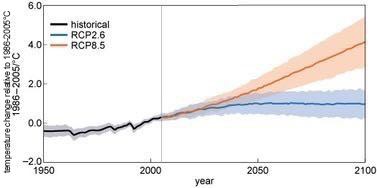
One approach is to use many different climate models instead of just one. This means that we have multiple predictions and can take, for example, the mean and the 90% range of these, as you saw for the GMST predictions in Session 4, (repeated in Figure 4).
Another way is to use multiple different versions of one model: changing the inputs slightly each time, to see the effect this has on the results. This is illustrated in the extract below from Tamsin Edwards’ (2015) work, published in the Guardian:
We used a computer model to simulate the Antarctic ice sheet from the recent past up to the year 2200: not just once, but 3000 times. Each version was slightly different to account for ‘known unknowns’ in the physical laws and simplifications describing how ice flows and slides, the map of the bedrock beneath the ice sheet, and when instability might be triggered in each region under [a] mid-high climate scenario…. This gave us a range of model predictions for sea level rise: three thousand possible futures fanning out from today.
If you are interested, you can participate in the citizen science project ‘climateprediction.net [Tip: hold Ctrl and click a link to open it in a new tab. (Hide tip)] ’, which uses the public’s spare computing power to run many different versions of climate models.
Using many climate models, or many versions of one climate model, broadens the simulated climate distributions. We can compare simulations of the past with observations to test whether the models were successful.

