

1 Climate models
Designing geoengineering requires the use of a model to predict its effects. How can models be used to inform both policy-makers and the public?
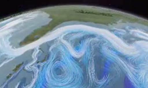
Video 1 is a stunning visualisation of the Earth system based on climate model simulations of the atmosphere, ocean and sea ice, and incorporating some observational data. It’s called ‘Dynamic Earth’, and is a visualisation based on the Goddard Earth Observing System (GEOS) atmospheric model and the MIT (Massachusetts Institute of Technology) general circulation model for the oceans and ice. First, flowing arrows show the patterns of air circulation, such as the Northern Hemisphere polar jet stream blowing from west to east; then whirls of blue show the eddies and streams of ocean circulation, with the Gulf Stream flowing along the coast of Florida to the North Atlantic.
-
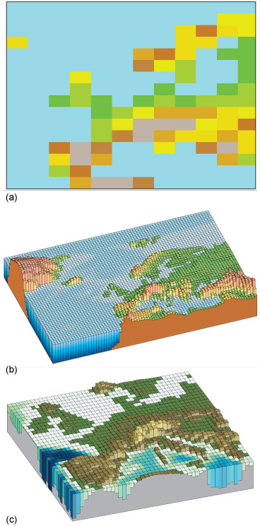
Why does it help in both weather and climate modelling to divide the world into grid squares?
-
The circulation of the atmosphere is very complex, and this breaks the problem down into a series of discrete and achievable tasks.
The smaller the size of grid squares in a climate model, the more detail can be included. The ‘Dynamic Earth’ video demonstrates some of the best examples of climate models available because they have large numbers of very small grid squares – we say, a very high resolution. (The resolution is the total number of points (pixels) within an image produced or displayed by the device.)
The ‘Ocean model’ used in Dynamic Earth is based on 2 332 800 grid squares. In contrast, the IPCC uses a low resolution model, equivalent to using a rather vintage-looking games console.
-
This may seem surprising: why could this be?
-
The greater the number of grid squares, the greater the number of calculations there are to make and so the slower the model is to run. Using a low-resolution model means it is possible to simulate longer time periods.
For all models apart from those using the lowest resolutions, the models are so slow to run that it is only practical to simulate time periods of a few months or years, even on a supercomputer – nowhere near the tens or hundreds of years needed for predicting climate – unless the area is restricted to a small region.
This is why IPCC (2013) global climate models have far lower resolutions than the stunning visualisations you saw in Figure 2.